Start with
possibilities.
Randomness gives a search process room to explore. The challenge is directing that exploration through a complicated energy landscape.
The PAOA story ↓Machine learning · Probabilistic computing
UC Santa Barbara · OPUS Lab ↗
Abdelrahman S. Abdelrahman
PhD candidate · Electrical & Computer Engineering
I work across the entire computing stack, from developing algorithms in Python and C++ to implementing them on specialized hardware such as FPGAs and single-photon avalanche diode arrays.
My research spans rigorous benchmarking of variational probabilistic algorithms such as PAOA against quantum counterparts such as QAOA. I also develop methods that learn how many samples stochastic neurons need to retain accuracy while substantially reducing memory use and computation. At the device level, I model stochastic processes in emerging technologies such as 2D memristors.
Beyond academia, I built real-time computer vision systems for safety monitoring and object tracking using PyTorch, YOLO, and ByteTrack. I worked from dataset preparation through deployment on resource-constrained NVIDIA Jetson devices.

01 / Research & publications
How can we learn better ways to search, sample, and compute? My work connects algorithms, stochastic devices, and physical systems.
Google Scholar ↗Randomness gives a search process room to explore. The challenge is directing that exploration through a complicated energy landscape.
The PAOA story ↓Learn the dynamics of a sampler, or learn the configurations it proposes. PAOA and IsingFormer approach the search process from complementary directions.
Learned proposals ↓Connect these algorithms to FPGA implementations, single-photon avalanche diode arrays, and configurable stochastic circuits.
From algorithm to SPAD array ↓
12 publications · figures, code & citations
Learning the dynamics of a sampler and learning the configurations it proposes.
Cool the model to favor low-energy states. Warm it up to explore more possibilities, and watch the sampled distribution take shape.
One-dimensional energy model.
Position in the energy landscape
Sampling from the current distribution.
Abdelrahman S. Abdelrahman1, Shuvro Chowdhury1, Flaviano Morone2, Kerem Y. Camsari1
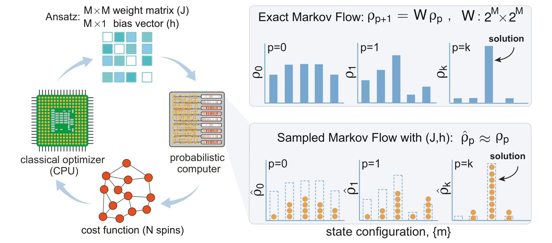
Can the dynamics of a probabilistic computer become the object of learning? Generalized PAOA parameterizes the couplings, fields, and schedules of a stochastic system, then improves them using sampled costs. The figures follow that idea from its mathematical construction to benchmarks and a learned annealing principle.
A classical optimizer updates the parameters that drive a probabilistic computer. Exact probability flow provides the theoretical description; independent samples provide a practical estimate when the state space becomes too large to enumerate.
The feedback loop. The classical optimizer updates couplings and biases; the probabilistic computer returns configurations from the resulting dynamics. The cost is evaluated from those samples, so the learned object is a search procedure rather than a single candidate solution.
 Expand figure ↗
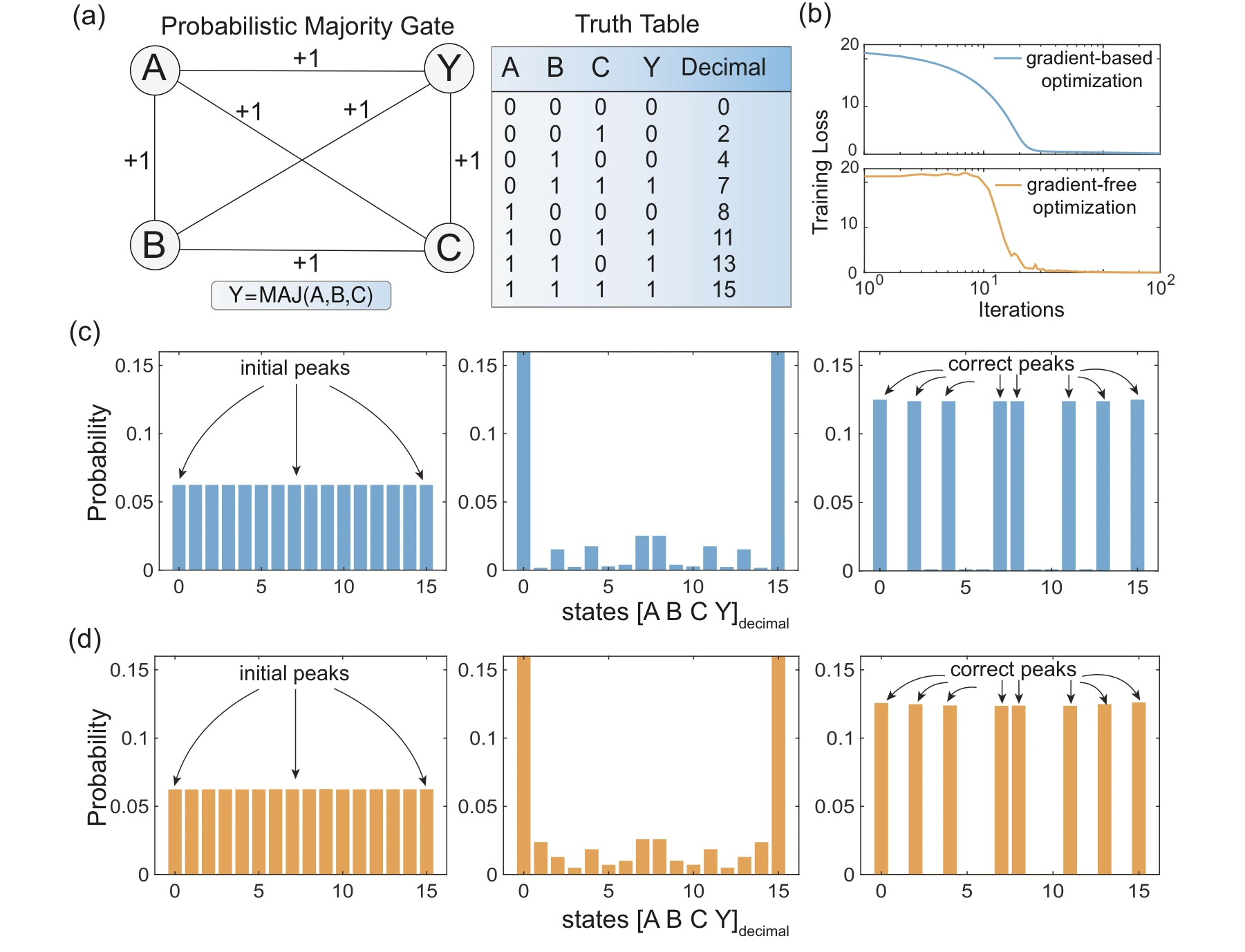
A four-node majority gate makes the target distribution small enough to inspect directly. Analytical and sample-based optimization reach matching outcomes, connecting the variational formulation to the sampling procedure used in larger systems.
Panels (a) and (b). The four-node majority gate provides a small problem with eight valid input–output combinations. The loss curves compare exact-gradient training with sample-based, gradient-free optimization, so both methods can be checked against the same known target.
Panels (c) and (d). Follow the probability assigned to each state over two layers. The exact Markov calculation is shown in (c); the MCMC approximation is shown in (d). Both concentrate probability on truth-table states rather than treating every configuration as equally likely.
 Expand figure ↗
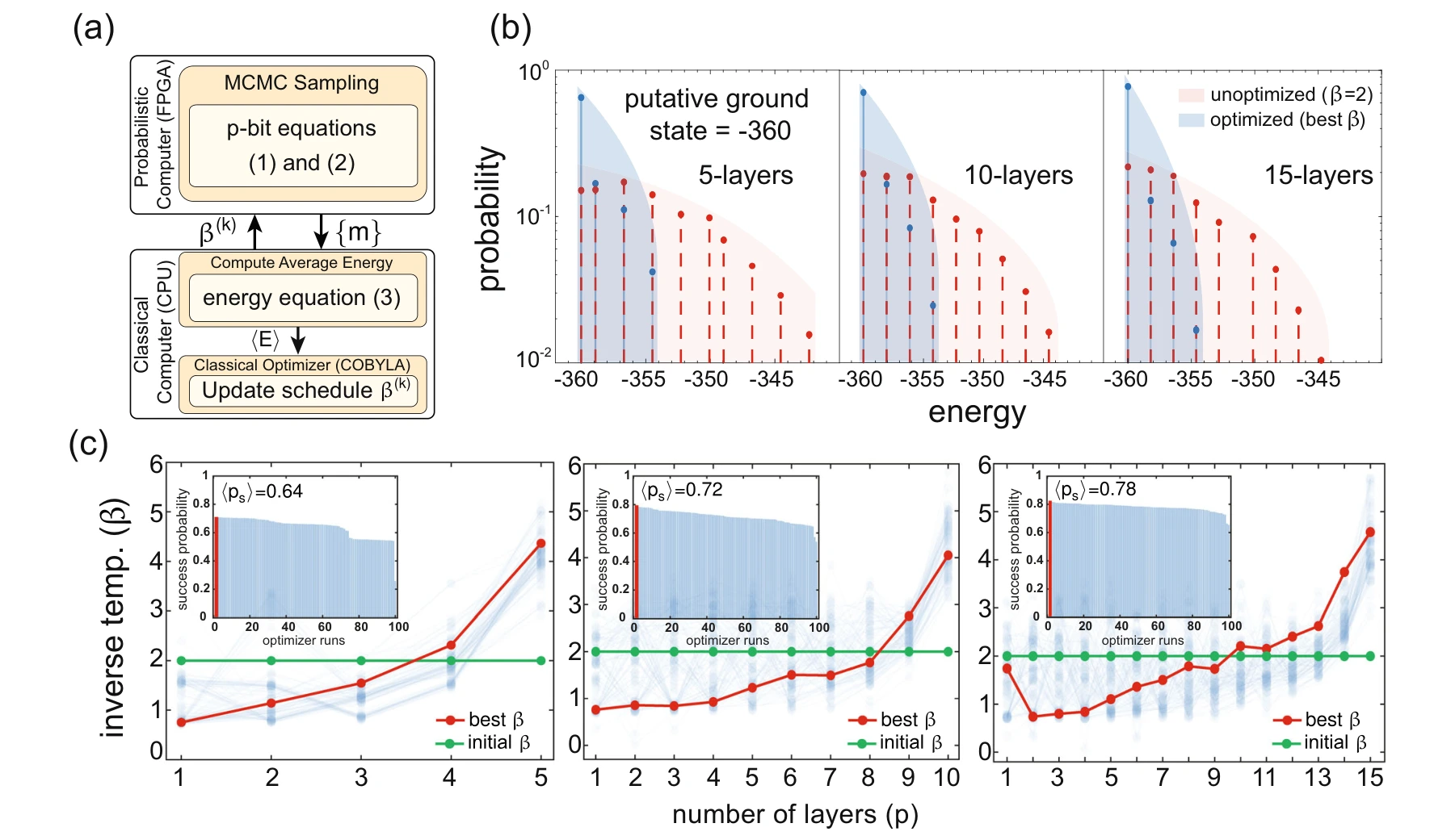
The next step moves from a small truth table to a three-dimensional spin glass. Optimizing the schedule on an FPGA-based probabilistic computer shifts the energy distribution toward lower-energy solutions and recovers an annealing-like trajectory.
Panels (a) and (b). The FPGA supplies configurations while a CPU updates the annealing schedule. The energy histogram compares the same spin-glass instance before and after optimization; the useful change is a larger concentration of samples near the putative ground state.
Panel (c). Schedules at depths 5, 10, and 15 start from the same flat inverse-temperature profile. The learned profiles resemble cooling schedules. The insets compare success probabilities across repeated optimization runs, exposing variation that a single best schedule would hide.
 Expand figure ↗
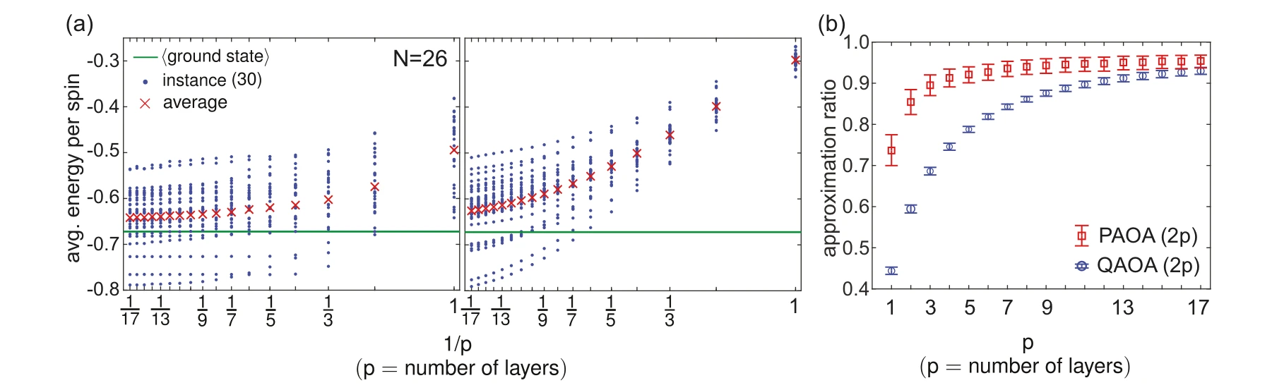
PAOA and QAOA are compared on the 26-spin Sherrington–Kirkpatrick model using matched parameter counts. The energy and approximation-ratio plots show how each method changes as the number of layers increases.
Panels (a) and (b). Panel (a) compares energy at matched parameter counts on 26-spin test instances. Panel (b) summarizes approximation ratios and bootstrap confidence intervals; PAOA schedules are transferred from a separate training set without retraining.
 Expand figure ↗
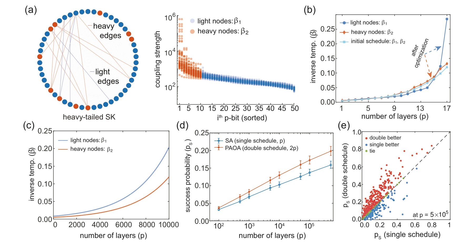
Heavy-tailed couplings create distinct groups of strongly and weakly connected spins. A two-schedule ansatz learns different temperature profiles for these groups, suggesting a problem-dependent annealing strategy that can be extended to larger depths.
Panels (a) and (b). Sorting the heavy-tailed couplings separates strongly and weakly connected spins. The two groups receive different learned schedules, making the comparison about the structure of the problem rather than simply increasing annealing depth.
Panels (c)–(e). The learned distinction motivates longer double schedules. The final panels compare average and instance-by-instance success against single-schedule simulated annealing, showing both aggregate performance and variation across the tested problems.
 Expand figure ↗
Putting it together
The progression connects a variational description, a controlled benchmark, hardware execution, and a learned scheduling rule. PAOA provides a framework for adapting the stochastic search process to the structure of the problem.
Abdelrahman, A. S., Chowdhury, S., Morone, F., & Camsari, K. Y. Generalized Probabilistic Approximate Optimization Algorithm. Nature Communications, 17, 498 (2026). https://doi.org/10.1038/s41467-025-67187-5
@article{abdelrahman2026paoa,
  title = {Generalized Probabilistic Approximate Optimization Algorithm},
  author = {Abdelrahman, Abdelrahman S. and Chowdhury, Shuvro and Morone, Flaviano and Camsari, Kerem Y.},
  journal = {Nature Communications},
  volume = {17},
  pages = {498},
  year = {2026},
  doi = {10.1038/s41467-025-67187-5}
}
Saleh Bunaiyan1,2, Corentin Delacour1, Shuvro Chowdhury1, Kyle Lee1, Abdelrahman S. Abdelrahman1, Kerem Y. Camsari1
Local Monte Carlo moves can struggle to traverse a rugged energy landscape. IsingFormer learns configurations at different temperatures and supplies global proposals to a parallel-tempering search. The paper first tests what the model learns, then studies spin glasses, reusable factorization encodings, and conditional scaling results.
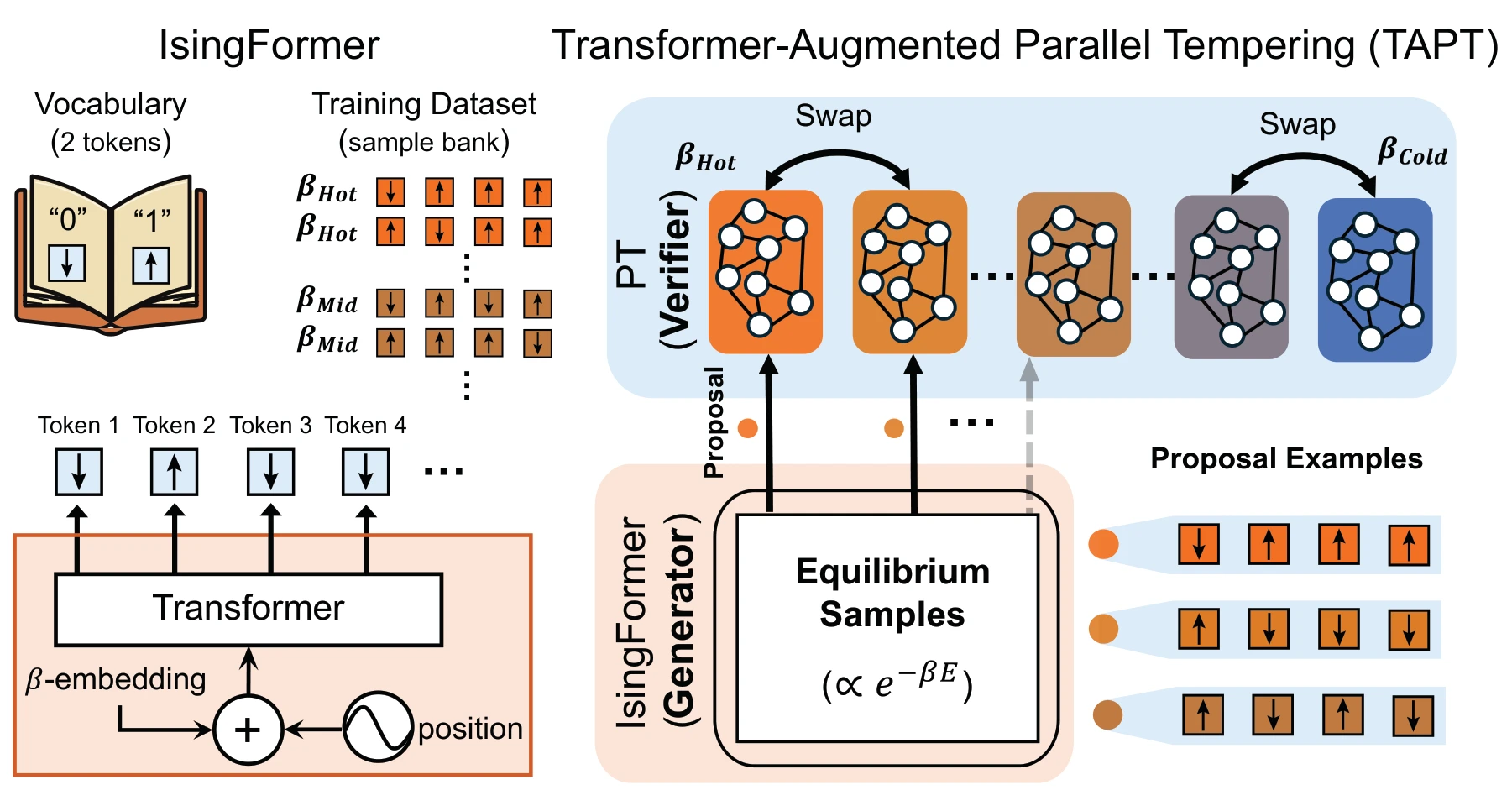
A temperature-conditioned Transformer learns from long-run MCMC configurations. It proposes complete configurations to selected replicas of a parallel-tempering ladder, where local updates and replica exchanges continue to propagate promising states.
Left: learning configurations. Long-run MCMC provides configurations at several inverse temperatures. A decoder-only Transformer learns a temperature-conditioned distribution over complete spin states, using both position information and a learned temperature embedding.
Right: using proposals. Generated configurations enter hot and intermediate replicas of a parallel-tempering ladder. Energy evaluation filters proposals, while local updates and replica swaps continue the search. The coldest replicas are not directly supplied with generated proposals.
 Expand figure ↗
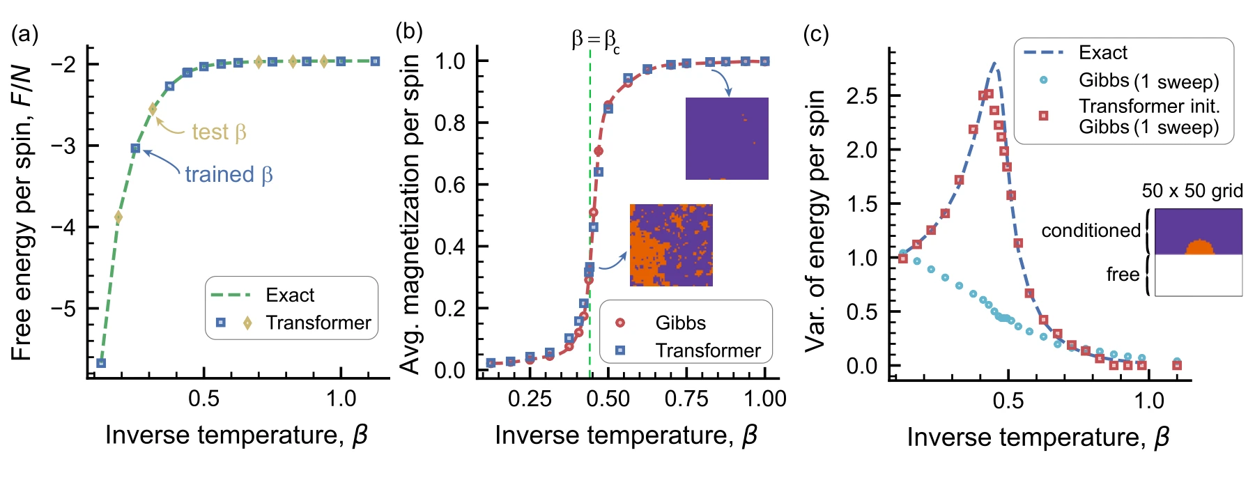
The two-dimensional Ising model offers physical quantities against which to check generated samples. Free energy, magnetization, and clamped-boundary examples test both interpolation to unseen temperatures and conditional generation outside the training setup.
Panels (a) and (b). Free energy tests interpolation between trained temperatures, while magnetization checks the finite-size transition. The comparison uses an exact free-energy reference and Gibbs samples, rather than relying on visual similarity alone.
Panel (c). The half-clamped boundary is absent from training. Energy variance after a single Gibbs sweep tests whether Transformer initialization helps under that changed condition.
 Expand figure ↗
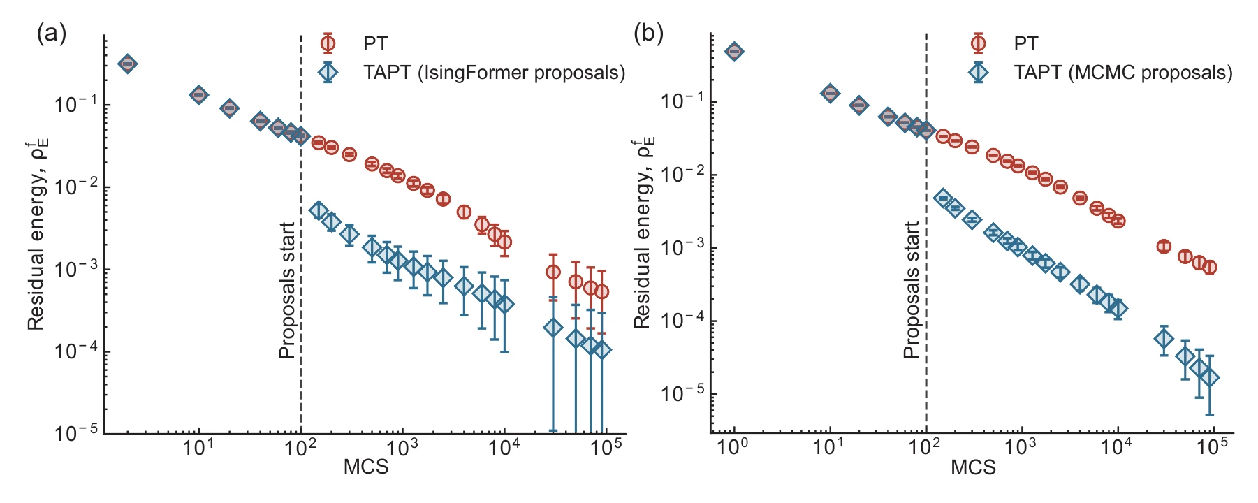
For three-dimensional spin-glass instances, the plots track residual energy against Monte Carlo sweeps. Turning on proposal moves changes the search trajectory relative to ordinary parallel tempering, with learned and MCMC-generated proposals compared separately.
Panels (a) and (b). The proposal source changes from IsingFormer to long-run MCMC. The dashed line marks activation after 100 sweeps, allowing the subsequent energy reduction to be compared with ordinary parallel tempering under each proposal source.
 Expand figure ↗
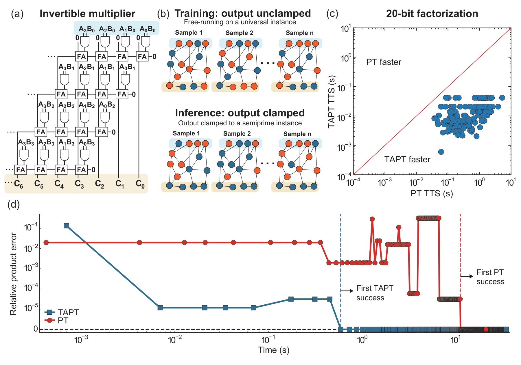
An invertible multiplier circuit encodes candidate factors and their product. Training with unclamped product spins creates a reusable generator; clamping a particular product later defines the search task for that target.
Panels (a) and (b). Clamping the product of an invertible multiplier turns factorization into an Ising search problem. Training uses an unclamped universal circuit; at inference, a target product conditions the search while the trained generator is reused.
Panels (c) and (d). The timing comparison covers 440 semiprime instances at a target success probability of 0.99. The example trajectory follows the relative product error for 1,022,117 = 1009 × 1013. The timing is conditional on an already-generated proposal bank.
 Expand figure ↗
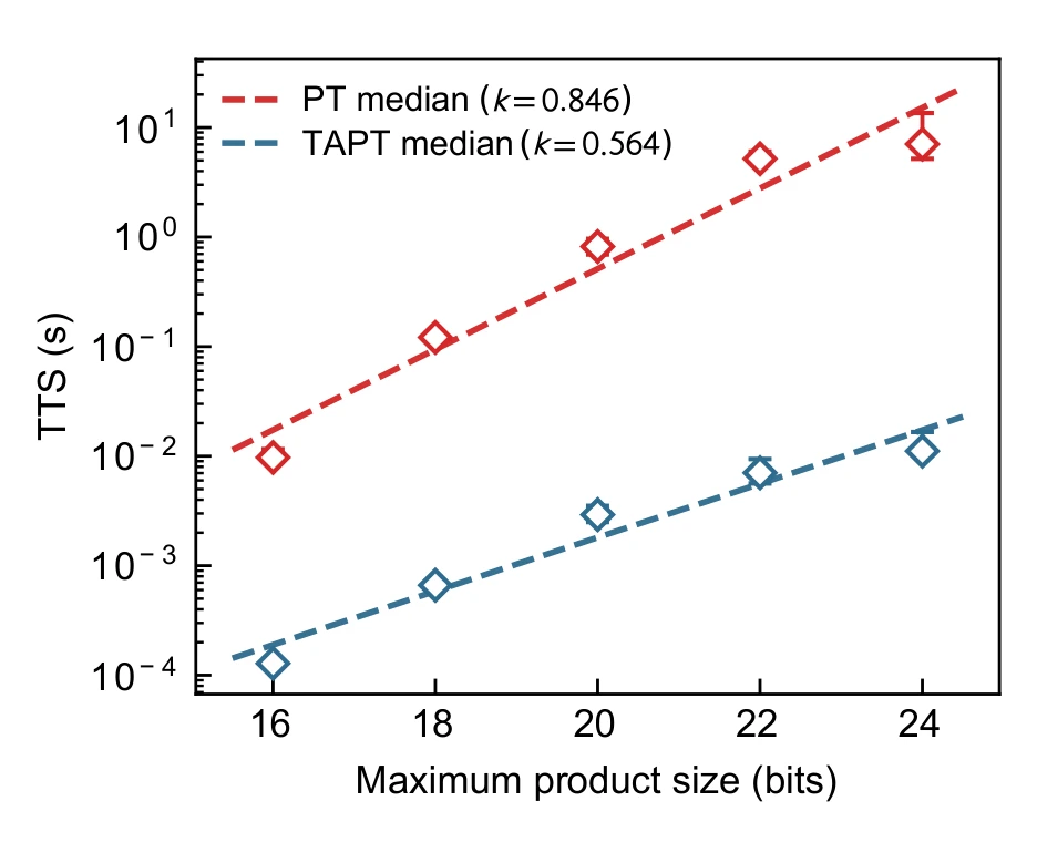
The scaling experiment measures time to solution conditional on pre-generated proposal banks. The fitted exponents compare the tested search procedures; generating those proposal banks is excluded, so this is not a claim of an end-to-end speedup including model training and generation.
Reading the axes. The horizontal axis is the maximum product bit length; the vertical axis is the median time to reach a 0.99 success probability. Markers summarize instances, error bars give bootstrap confidence intervals, and dashed lines show exponential fits.
What is timed. This experiment uses proposals generated by long-run MCMC, rather than IsingFormer. Optimization operations are included, but offline proposal-bank generation is excluded. The fitted exponents, 0.846 for PT and 0.564 for TAPT, describe this conditional comparison.
 Expand figure ↗
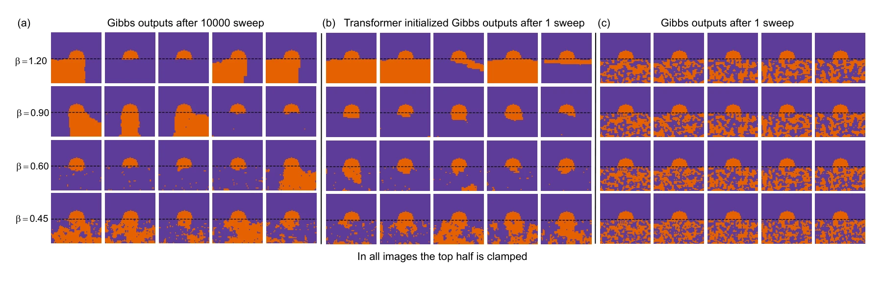
Spin configurations compare Transformer and random initialization when part of the lattice is clamped. The test probes whether learned context helps the subsequent Monte Carlo evolution.
Panels (a)–(c). The long-run reference is compared with one sweep after Transformer initialization and one sweep from random initialization. Similar-looking configurations suggest a useful starting state, but do not by themselves establish convergence.
 Expand figure ↗
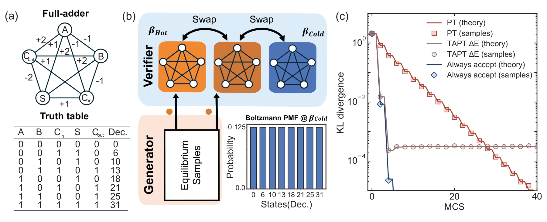
A small full-adder system makes the stationary distribution directly inspectable. The example shows why energy-only acceptance of external proposals does not generally preserve the Boltzmann target.
Panels (a) and (b). A five-spin full-adder and a controlled three-replica ladder make the target distribution exactly inspectable. Proposals are supplied to two replicas, leaving the coldest replica unaugmented.
Panel (c). The nonzero limiting KL divergence under the energy-only acceptance rule exposes its sampling bias. Exact transition-matrix results and Monte Carlo estimates distinguish optimization usefulness from unbiased equilibrium sampling.
 Expand figure ↗
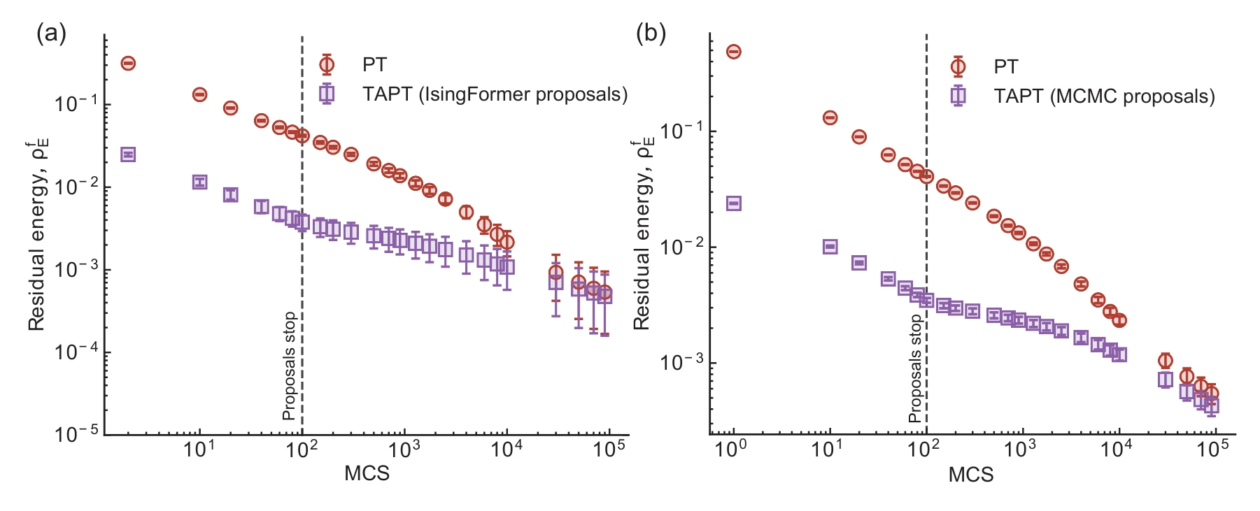
The warm-start experiment enables proposals only for the first part of the run. The later trajectories test whether an early advantage persists when the search returns to ordinary parallel tempering.
Panels (a) and (b). Both proposal sources are switched off after the initial 100 sweeps. The later approach toward the PT baseline tests whether the early advantage survives without continued proposal moves.
 Expand figure ↗
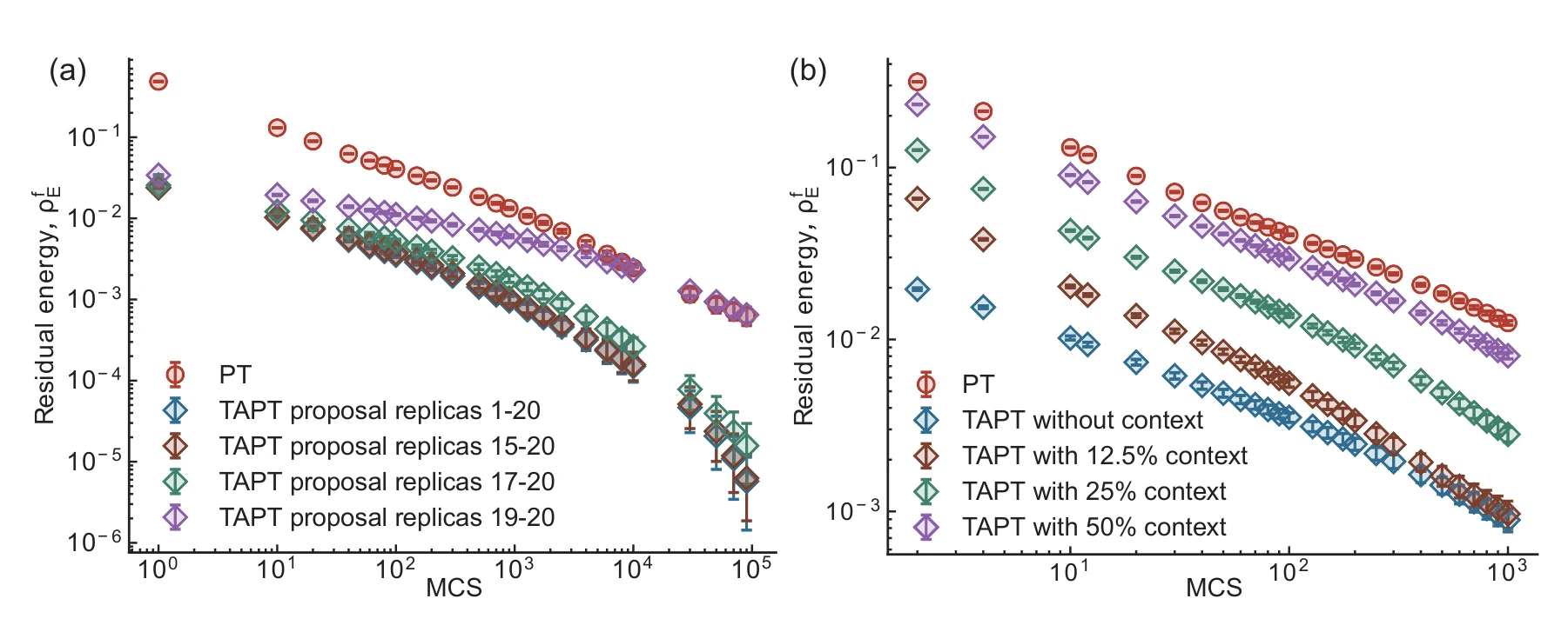
Ablations change which replicas receive proposals and how their context is chosen. These experiments isolate design choices in the proposal mechanism using MCMC-generated configurations.
Panels (a) and (b). The first ablation changes which replicas receive proposals; the second changes how much of the current state conditions a proposal. Both use MCMC-generated candidates, isolating these choices from Transformer training.
 Expand figure ↗
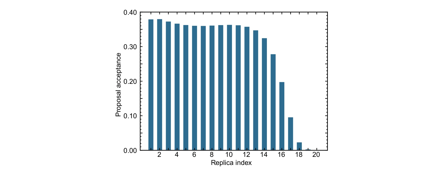
Acceptance varies across the parallel-tempering ladder. The per-replica plot shows where global candidates are accepted and where the existing configurations are harder to replace.
Reading the replica index. Indices run from hotter to colder replicas. The plot covers proposal-enabled replicas 1–20; replicas 21 and 22 receive no proposals, so there is no acceptance-rate measurement for them here.
 Expand figure ↗
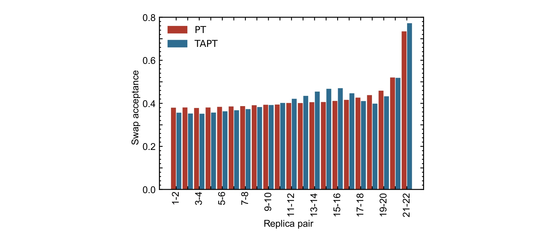
Swap-acceptance probabilities compare ordinary and augmented parallel tempering. This checks how the added proposal moves affect the exchange pathway through the temperature ladder.
What is compared. The curves measure exchanges between adjacent replicas, combining the alternating swap stages. Their broad similarity checks whether adding proposals substantially changes this communication pathway in the tested ladder.
 Expand figure ↗
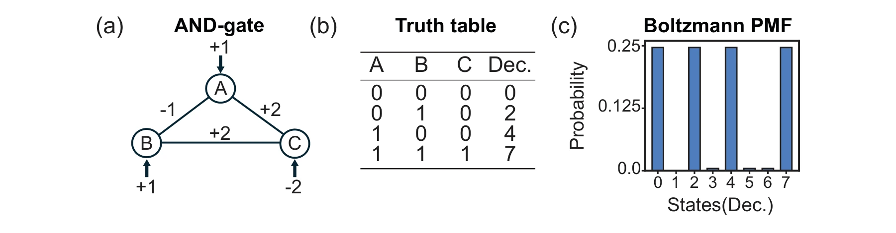
The three-spin AND-gate model provides an exactly enumerable example. Its truth table and Boltzmann probabilities connect the circuit encoding to the intended target distribution.
Panels (a)–(c). The Ising graph, truth table, and eight-state distribution connect the encoding to the logical constraint. States 0, 2, 4, and 7 satisfy the AND relation and receive the largest probabilities.
 Expand figure ↗
Putting it together
The generator and Monte Carlo search play complementary roles. The energy-only proposal rule is used here as an optimization heuristic; the supplementary analysis explains why unbiased equilibrium sampling requires a fuller correction.
Bunaiyan, S., Delacour, C., Chowdhury, S., Lee, K., Abdelrahman, A. S., & Camsari, K. Y. Isingformer: Augmenting parallel tempering with learned proposals. Under review (2026). arXiv:2509.23043.
@misc{bunaiyan2026isingformer,
  title = {Isingformer: Augmenting parallel tempering with learned proposals},
  author = {Bunaiyan, Saleh and Delacour, Corentin and Chowdhury, Shuvro and Lee, Kyle and Abdelrahman, Abdelrahman S. and Camsari, Kerem Y.},
  year = {2026},
  eprint = {2509.23043},
  archivePrefix = {arXiv},
  primaryClass = {cs.LG},
  url = {https://arxiv.org/abs/2509.23043}
}
Corentin Delacour1, Xiuqi Zhang1, Abdelrahman S. Abdelrahman1, Saleh Bunaiyan1,2, Kyle Lee1, Shuvro Chowdhury1, Kerem Y. Camsari1
Which algorithms can move between Ising platforms, and where does the hardware change the algorithm itself? This review uses a co-design perspective to connect problem encoding, sampling methods, capacity limits, variational optimization, and generative AI. Its four figures form a map of those connections.
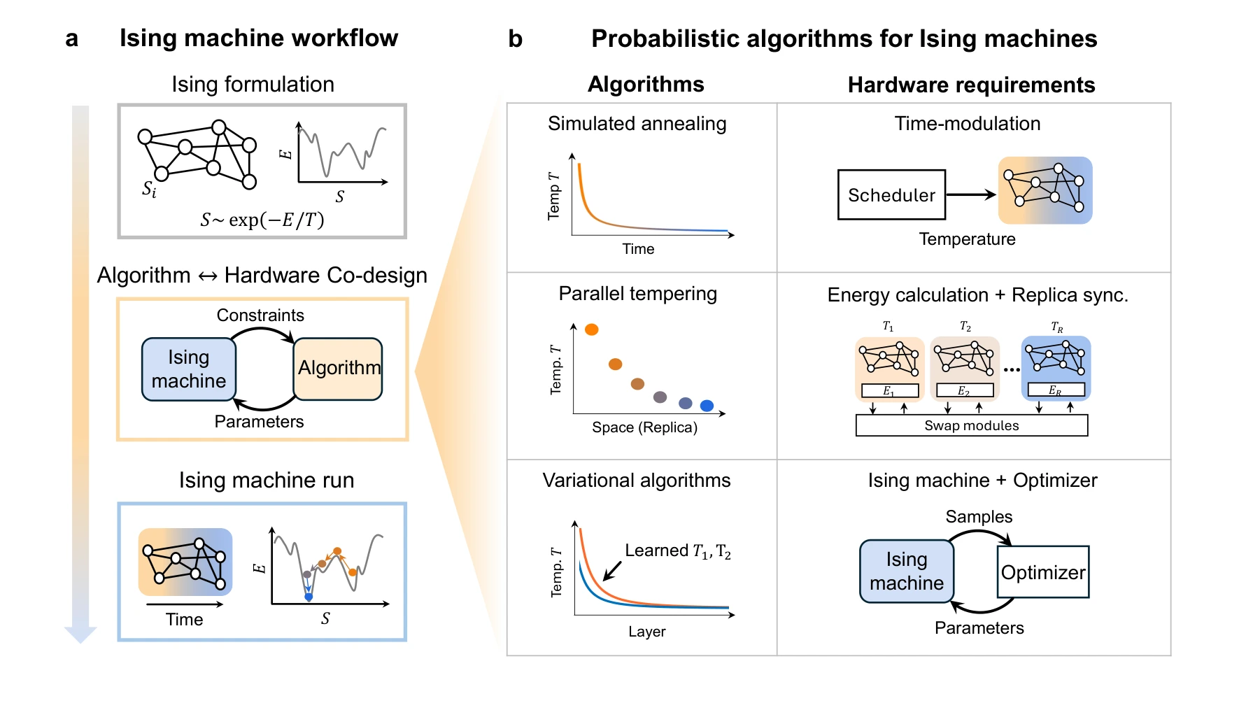
A task is encoded as an Ising energy landscape, an algorithm drives exploration, and samples are evaluated against the original objective. Hardware capabilities constrain this loop while new algorithms create demands for different hardware features.
Panel (a). The task is encoded as an energy function before the machine explores configurations. Hardware constraints and algorithmic requirements feed back into one another, so the workflow includes both problem formulation and physical execution.
Panel (b). The three algorithm families place different demands on hardware: annealing needs temperature scheduling, tempering needs replica exchange and energy calculations, and variational methods need sampled feedback to a classical optimizer.
 Expand figure ↗
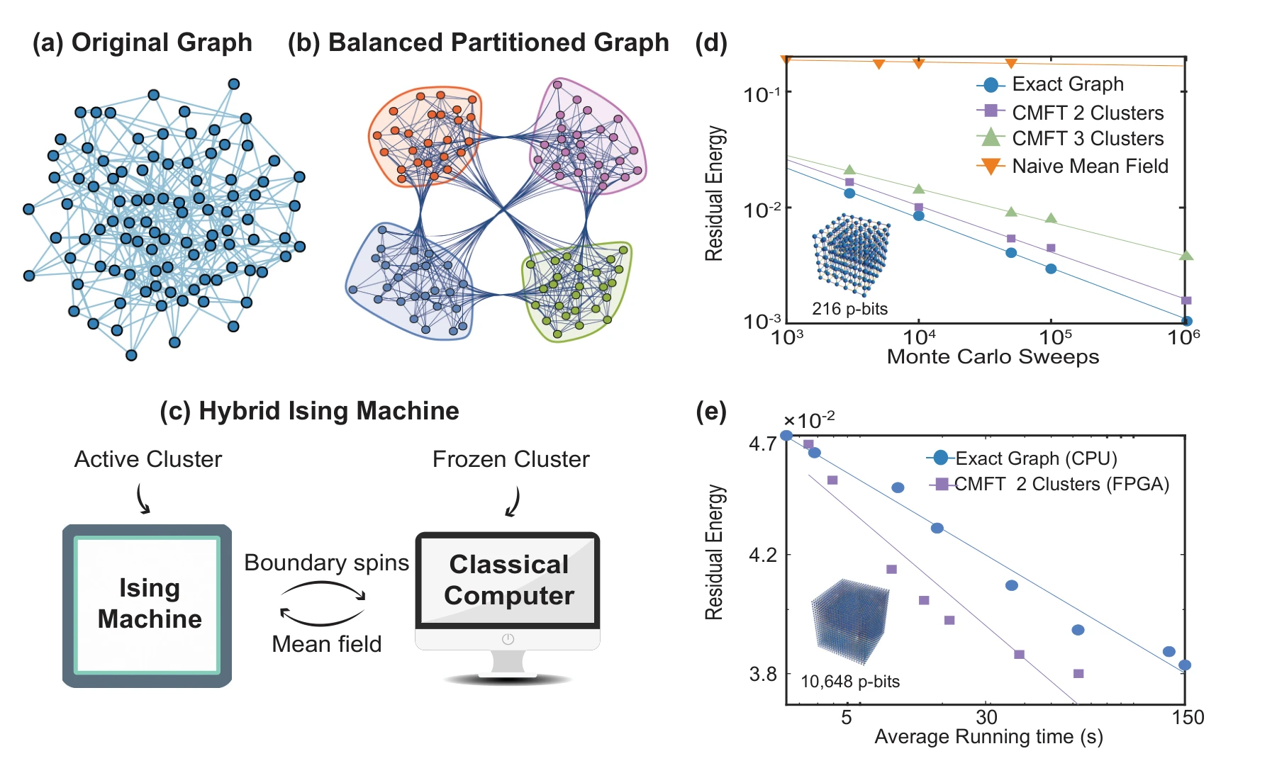
Cluster mean-field methods partition a large interaction graph into hardware-sized pieces. The figure contrasts serial and parallel updates, showing how classical processing approximates interactions at the boundaries between clusters.
Panels (a)–(c). The interaction graph is partitioned into hardware-sized clusters. An active cluster is updated while the remaining clusters are frozen, and a classical processor approximates interactions across their boundaries.
Panels (d) and (e). CPU curves compare convergence as the cluster count changes. The FPGA comparison then tests a larger problem than one device can hold, separating a capacity-scaling method from a claim about arbitrary partitioning being equally effective.
 Expand figure ↗
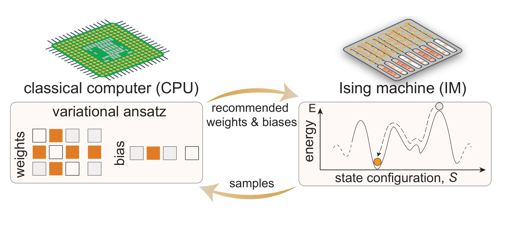
PAOA adds a learnable layer to the workflow. Costs estimated from samples update effective couplings, fields, or schedules, creating a sequence of stochastic dynamics adapted to the optimization problem.
The two sides of the loop. The CPU evaluates the sampled objective and changes variational parameters. The Ising machine returns states under those parameters; repeating the exchange learns a non-equilibrium trajectory rather than assuming a fixed thermal distribution.
 Expand figure ↗
The relationship works in both directions: samples from probabilistic systems can train generative models, while learned models can propose global configurations for search. The generator–verifier view helps distinguish proposing a candidate from evaluating its quality.
Training and search. The left side supplies temperature-indexed MCMC data for the generator. The right side inserts complete generated configurations into a tempering search, where proposal evaluation and replica exchange remain necessary. The acceptance rule determines whether the resulting process is suitable for equilibrium sampling or optimization.
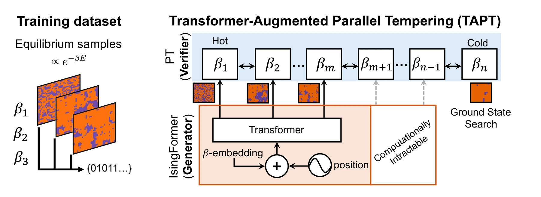 Expand figure ↗
Putting it together
The figures move from the basic workflow to capacity scaling, learned dynamics, and generative proposals. Together they explain why probabilistic computing benefits from developing algorithms and physical implementations in conversation with one another.
Delacour, C., Zhang, X., Abdelrahman, A. S., Bunaiyan, S., Lee, K., Chowdhury, S., & Camsari, K. Y. Probabilistic algorithms for Ising machines from optimization to generative AI. Nature Reviews Electrical Engineering (2026). https://doi.org/10.1038/s44287-026-00344-0
@article{delacour2026probabilistic,
  title = {Probabilistic algorithms for Ising machines from optimization to generative AI},
  author = {Delacour, Corentin and Zhang, Xiuqi and Abdelrahman, Abdelrahman S. and Bunaiyan, Saleh and Lee, Kyle and Chowdhury, Shuvro and Camsari, Kerem Y.},
  journal = {Nature Reviews Electrical Engineering},
  year = {2026},
  doi = {10.1038/s44287-026-00344-0}
}
Connecting probabilistic algorithms to devices and reusable circuit architectures.
Each bit takes the value 0 or 1. Adjust the bias to change its probability and watch many independent bits respond.
p-bit model · dimensionless bias.
Sampling independent bits.
Ziyad Alswaidan1, Abdelrahman S. Abdelrahman2, Md Sakibur Sajal1, Shuvro Chowdhury2, Kai-Chun Lin1, Hunter Guthrie1, Sanjay Seshan1, Shawn Blanton1, Flaviano Morone3, Marc Dandin1, Kerem Y. Camsari2, Tathagata Srimani1
A hardware sampler rarely behaves like an ideal mathematical activation function. This work asks whether variational optimization can operate with the asymmetric responses and variability of real SPAD devices. The story moves from the physical platform to characterization, algorithm tests, and deeper simulated schedules.
The hardware–software loop combines a classical optimizer, cost evaluations, and samples from a 64 × 64 perimeter-gated SPAD array. The chip and board photographs place the algorithm alongside the physical platform and its nonuniform device responses.
Panel (a). The optimizer receives a cost estimated from sampled configurations and updates the PAOA parameters. This is the algorithmic loop that the physical sampler supports.
Panels (b) and (c). The die view shows distinct device activation curves, while the board photograph places the array alongside its control and readout circuitry. Their separation makes device variability visible within the system architecture.
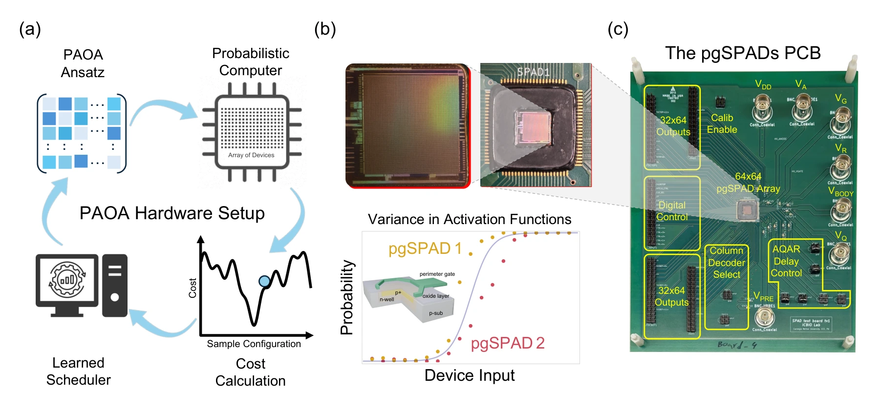 Expand figure ↗
Gate voltage changes the dark-count behavior of each device. Quenching, reset, and a defined integration window turn those stochastic events into binary outputs; their averaged response reveals the activation function available to the algorithm.
Panels (a) and (b). The perimeter gate changes the electric field near the SPAD junction edge. The readout circuit then converts avalanche events into a bit: at least one event within the integration window gives one output state, while no event gives the other.
Panels (c) and (d). The time traces show how gate voltage changes switching statistics. The measured activation curves compare devices, rather than repeated measurements of one ideal element; the Gompertz fit describes their asymmetric average response.
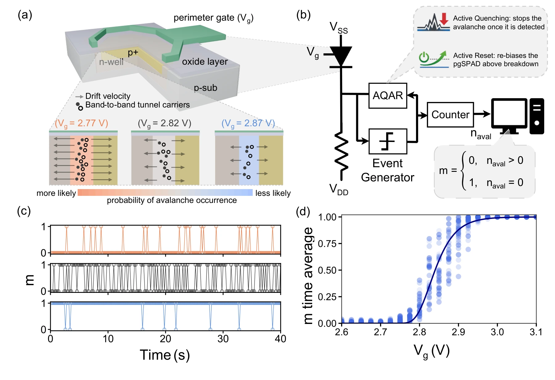 Expand figure ↗
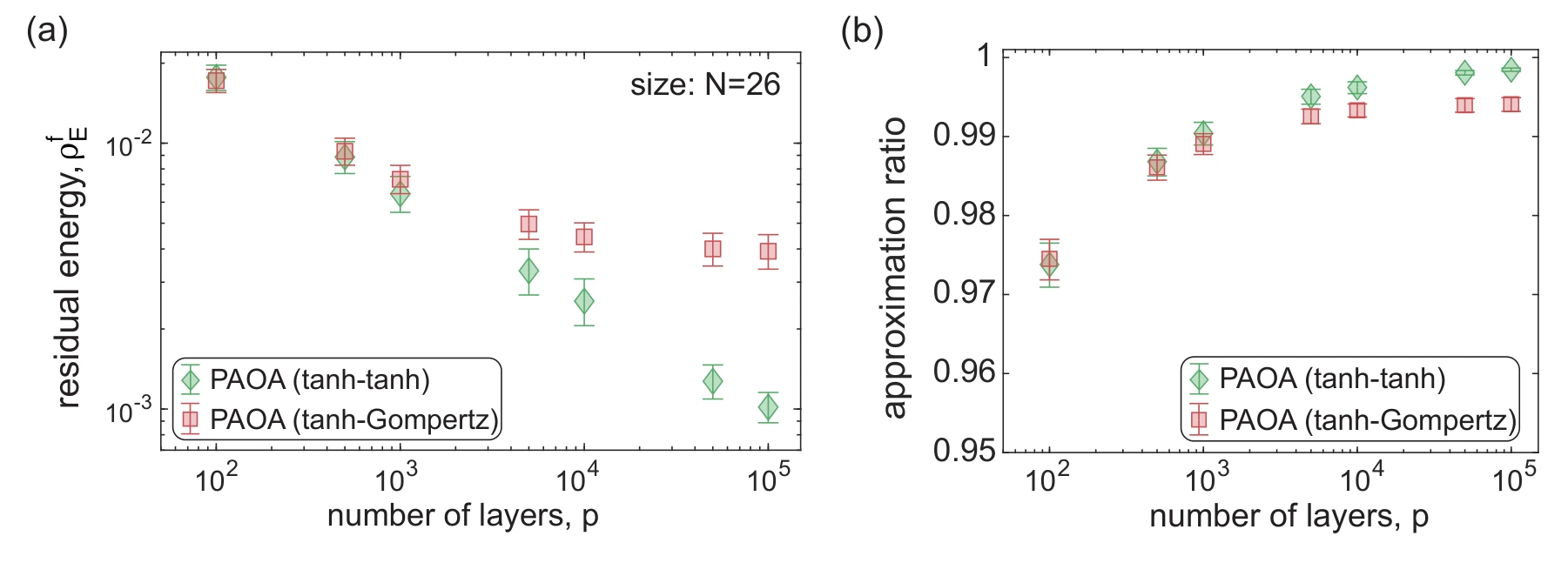
The benchmarks separate activation mismatch from matched hardware deployment. They compare idealized tanh and asymmetric Gompertz responses, then place measured SPAD inference alongside simulation using a hardware-matched training model.
Panels (a) and (b). Residual energy and approximation ratio compare matched tanh training/inference with tanh training followed by Gompertz inference. The schedules are learned on training instances and applied to a separate test set without retraining.
Panels (c) and (d). These panels instead use matched Gompertz schedules for both hardware and CPU inference. The hardware averages 50 runs, compared with one million in simulation. Bootstrap confidence intervals help distinguish agreement from sampling variability.
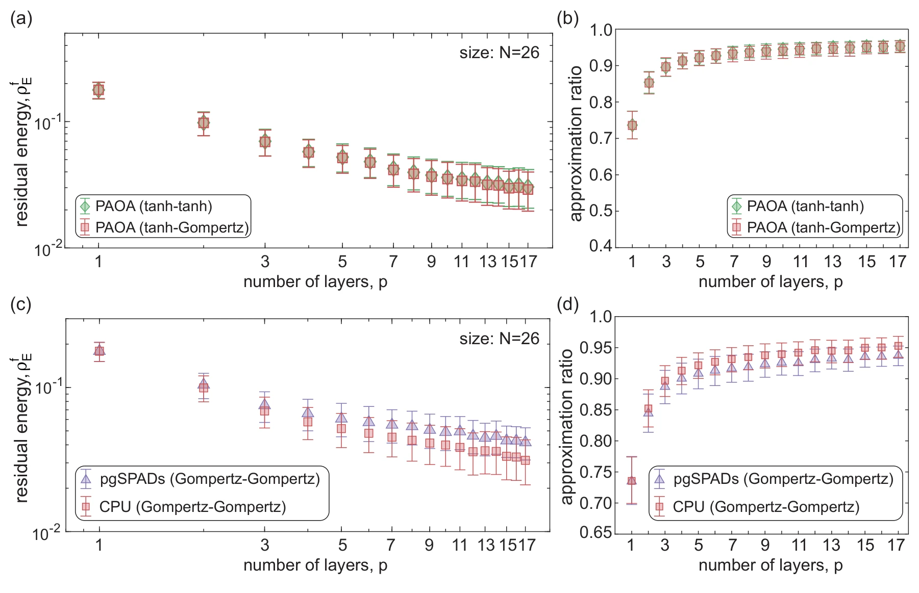 Expand figure ↗
CPU simulations extrapolate schedules learned at shallow depth to much longer runs. Residual energy and approximation ratio track the resulting improvement. These large-depth curves are simulations, rather than additional measurements on the physical array.
Panels (a) and (b). The same extrapolated schedules are evaluated using residual energy and approximation ratio. They were learned at depth 17 and extended without retraining; these large-depth results are CPU simulations, with confidence intervals across the tested instances and runs.
 Expand figure ↗
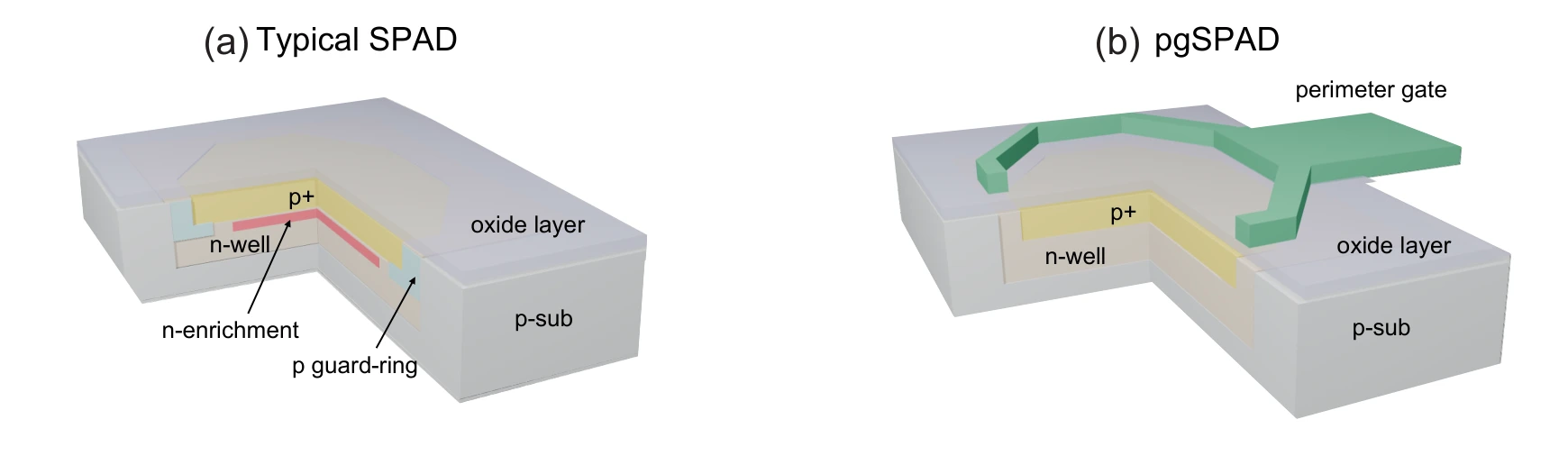
Cross-sections contrast a conventional SPAD with its perimeter-gated variant. The gate provides a way to influence the junction-edge electric field and the resulting stochastic behavior.
Panels (a) and (b). The cross-sections compare a conventional SPAD with the added perimeter gate. That gate provides a separate way to influence the junction-edge field.
 Expand figure ↗
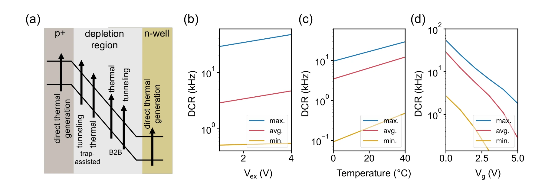
The panels relate carrier-generation mechanisms to bias voltage, temperature, and gate voltage. These measurements explain why a device’s probabilistic response changes with its environment.
Panel (a) and panels (b)–(d). Carrier-generation mechanisms are followed by measured dark-count rates versus excess bias, temperature, and gate voltage. Minimum, maximum, and mean curves expose variation across the array.
 Expand figure ↗
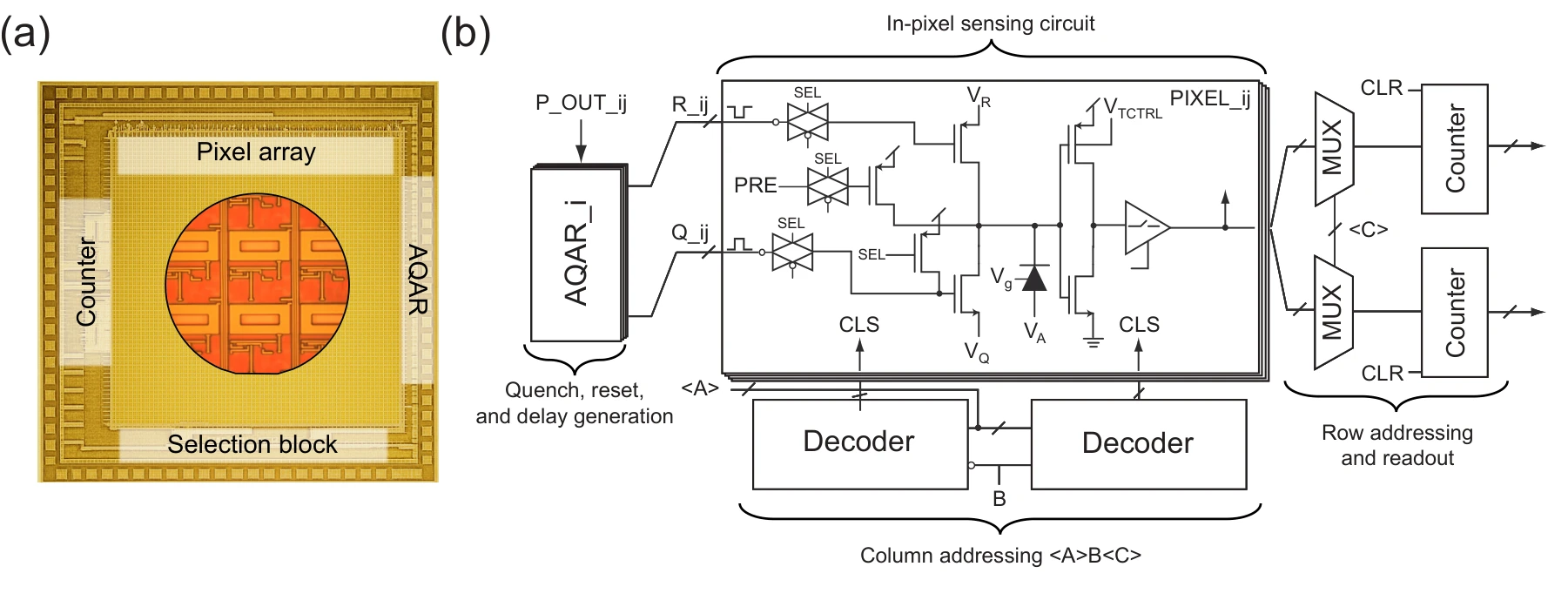
The photomicrograph and circuit schematic connect the 64 × 64 array to the addressing, quenching, reset, and readout functions required for characterization.
Panels (a) and (b). The micrograph identifies the array on the die. The circuit diagram shows the addressing, quench/reset, and counter blocks that make individual-pixel characterization possible.
 Expand figure ↗
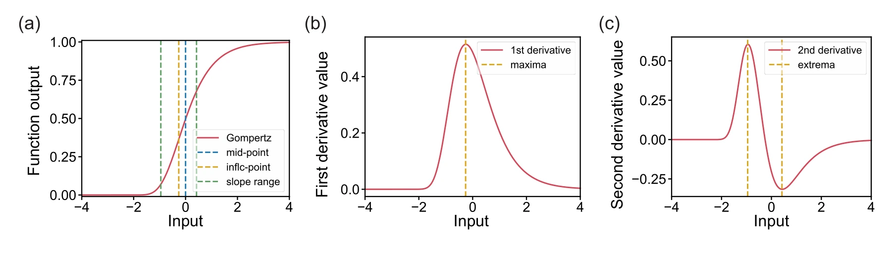
The Gompertz response and its derivatives identify the midpoint, inflection point, and transition range. They provide interpretable quantities for modeling the measured activation curves.
Panels (a)–(c). The activation curve and its first two derivatives distinguish the midpoint, inflection point, and transition range of the asymmetric Gompertz response.
 Expand figure ↗
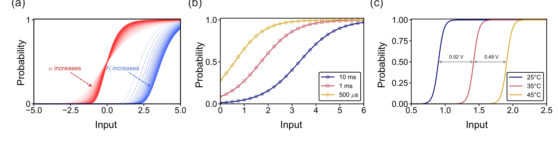
Simulations and measurements show how slope and midpoint change across device parameters, integration windows, and temperature. These effects motivate activation-aware learning.
Panels (a)–(c). Simulation separates slope changes from midpoint shifts. Measurements then show how integration time and temperature alter the effective activation curve, alongside manufacturing variability.
 Expand figure ↗
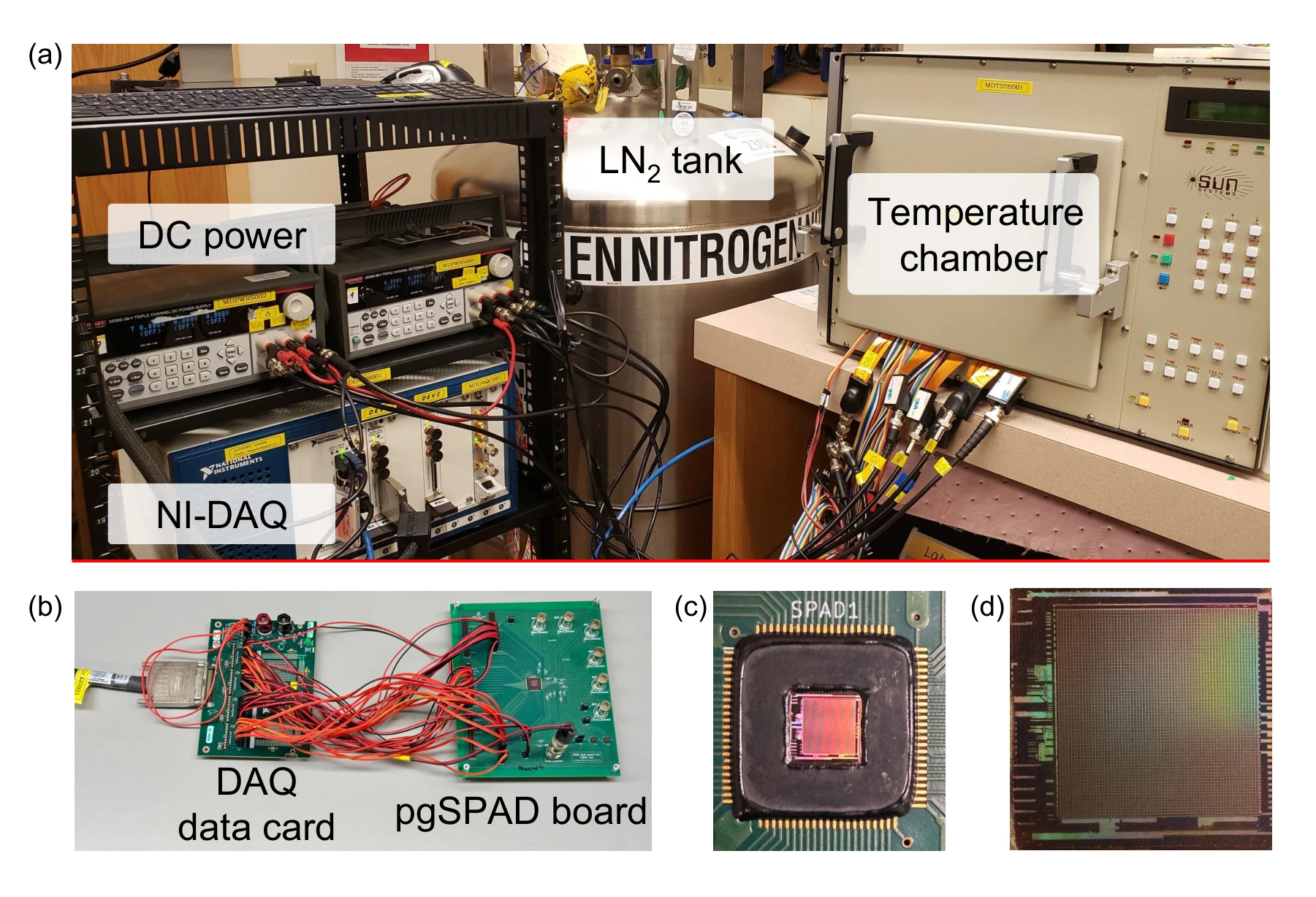
The temperature chamber, data-acquisition equipment, board, and die connect the reported device responses to the actual measurement setup.
Panels (a) and (b). The temperature chamber, liquid-nitrogen tank, and power supplies establish the operating conditions. The data-acquisition setup supplies timing signals and records the device output, connecting the characterization curves to a physical measurement procedure.
Panels (c) and (d). The board photograph shows the wire-bonded chip and protected connections. The micrograph locates the 64 × 64 array and its peripheral logic. These are different views of the same measurement platform, from laboratory equipment down to the die.
 Expand figure ↗
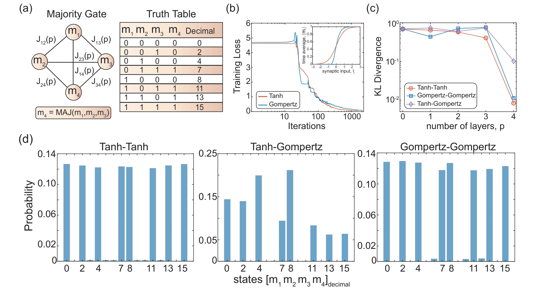
A majority-gate benchmark compares matched tanh and Gompertz learning with mismatched inference. The loss, divergence, and final state distributions make the effect of activation choice visible.
Panels (a) and (b). The majority-gate network and its valid truth-table states define an exactly inspectable target. The training curves then compare learning with symmetric tanh and asymmetric Gompertz activations.
Panels (c) and (d). KL divergence and the final state probabilities distinguish matched training/inference from activation mismatch. Comparing these two panels checks both a scalar error measure and which configurations receive probability at the final depth.
 Expand figure ↗
Putting it together
The experiments connect device characterization to the optimization procedure. They support using a model of the hardware response during learning instead of assuming that every physical stochastic element implements an ideal tanh function.
Alswaidan, Z., Abdelrahman, A. S., Sajal, M. S., Chowdhury, S., Lin, K.-C., Guthrie, H., Seshan, S., Blanton, S., Morone, F., Dandin, M., Camsari, K. Y., & Srimani, T. Probabilistic approximate optimization using single-photon avalanche diode arrays. npj Unconventional Computing, in press (2026).
@article{alswaidan2026spad,
  title = {Probabilistic approximate optimization using single-photon avalanche diode arrays},
  author = {Alswaidan, Ziyad and Abdelrahman, Abdelrahman S. and Sajal, Md Sakibur and Chowdhury, Shuvro and Lin, Kai-Chun and Guthrie, Hunter and Seshan, Sanjay and Blanton, Shawn and Morone, Flaviano and Dandin, Marc and Camsari, Kerem Y. and Srimani, Tathagata},
  journal = {npj Unconventional Computing},
  year = {2026},
  note = {In press},
  eprint = {2602.13943},
  archivePrefix = {arXiv},
  url = {https://arxiv.org/abs/2602.13943}
}
Saleh Bunaiyan1,2, Mohammad Alsharif3,4, Abdelrahman S. Abdelrahman1, Hesham ElSawy5, Suraj S. Cheema6, Suhaib A. Fahmy4, Kerem Y. Camsari1, Feras Al-Dirini5,6
Can a stochastic neuron be designed as reusable parts rather than a tightly coupled circuit? This work separates the source of randomness from the input and activation paths. The figures develop the architecture, demonstrate configurable responses, and test how sharing stochastic units affects a digital implementation.
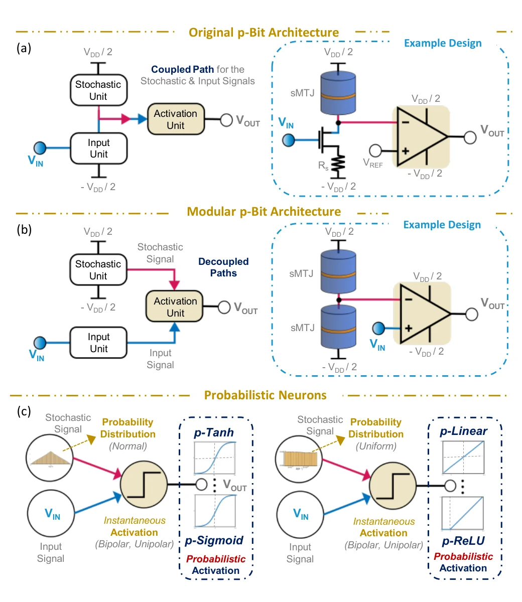
The opening architecture contrasts a coupled p-bit with a modular design. Decoupling the stochastic and activation units makes it possible to change the neuron response without rebuilding the entire source of randomness.
Panel (a). In the original architecture, the stochastic element and input path meet within the same circuit. Changing the random source or its response can therefore also affect how the input is processed.
Panel (b). The modular architecture separates the stochastic unit from the input and activation paths. The dual-sMTJ example supplies randomness to a distinct activation circuit, giving the designer separate choices for these two functions.
Panel (c). The lower diagrams connect a random-variable distribution and an instantaneous activation function to the time-averaged neuron response. The point is configurability: different combinations can produce probabilistic tanh, sigmoid, ReLU, or linear behavior.
 Expand figure ↗
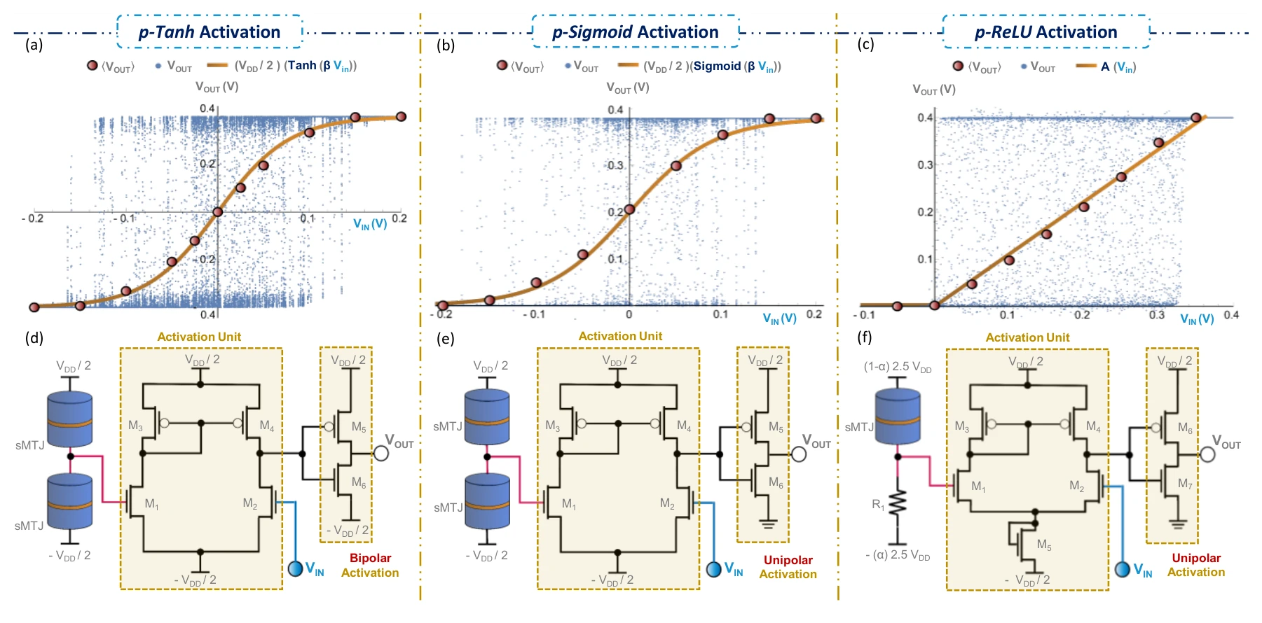
Spintronic circuit examples implement probabilistic versions of tanh, sigmoid, and ReLU. Instantaneous outputs and time-averaged responses connect transistor-level designs to the activation functions they realize.
Panels (a)–(c). Instantaneous responses and time averages are shown separately for probabilistic tanh, sigmoid, and ReLU neurons. The average activation is the quantity to compare with the intended nonlinear function.
Panels (d)–(f). The corresponding transistor-level designs change the activation circuit and stochastic unit. Comparing each circuit with the response directly above it connects the modular design choices to the measured behavior.
 Expand figure ↗
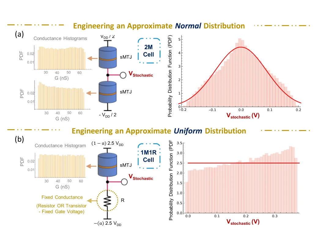
Different stochastic-unit constructions produce different voltage distributions. The normal-like and uniform-like examples show how this module can be selected to support the desired probabilistic activation.
Panel (a). Two stochastic magnetic tunnel junctions form a voltage divider. The conductance histograms on the left describe the individual elements; the voltage histogram on the right shows the approximately normal distribution produced by the combined stochastic unit.
Panel (b). Replacing one junction with a fixed resistor changes the output distribution to approximately uniform. Comparing the two rows shows why the stochastic unit is a design choice: its distribution helps determine the neuron’s eventual activation function.
 Expand figure ↗
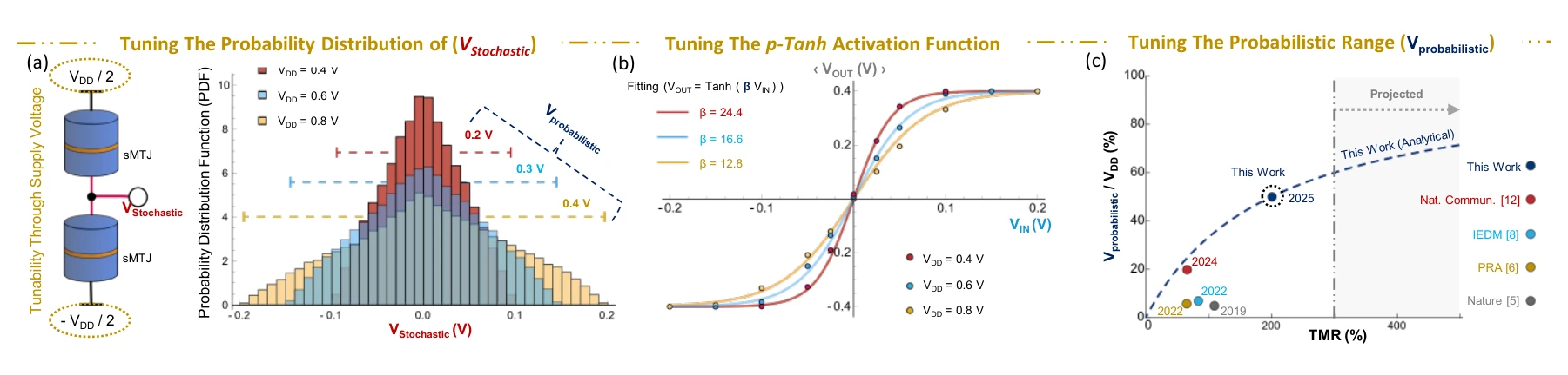
The response is not fixed by the architecture alone. Supply conditions and device characteristics change the transition range, providing circuit-level controls over the resulting activation function.
Panels (a)–(c). Supply voltage tunes the stochastic distribution, β scales the tanh response, and the final plot relates the available probabilistic range to tunneling magnetoresistance.
 Expand figure ↗
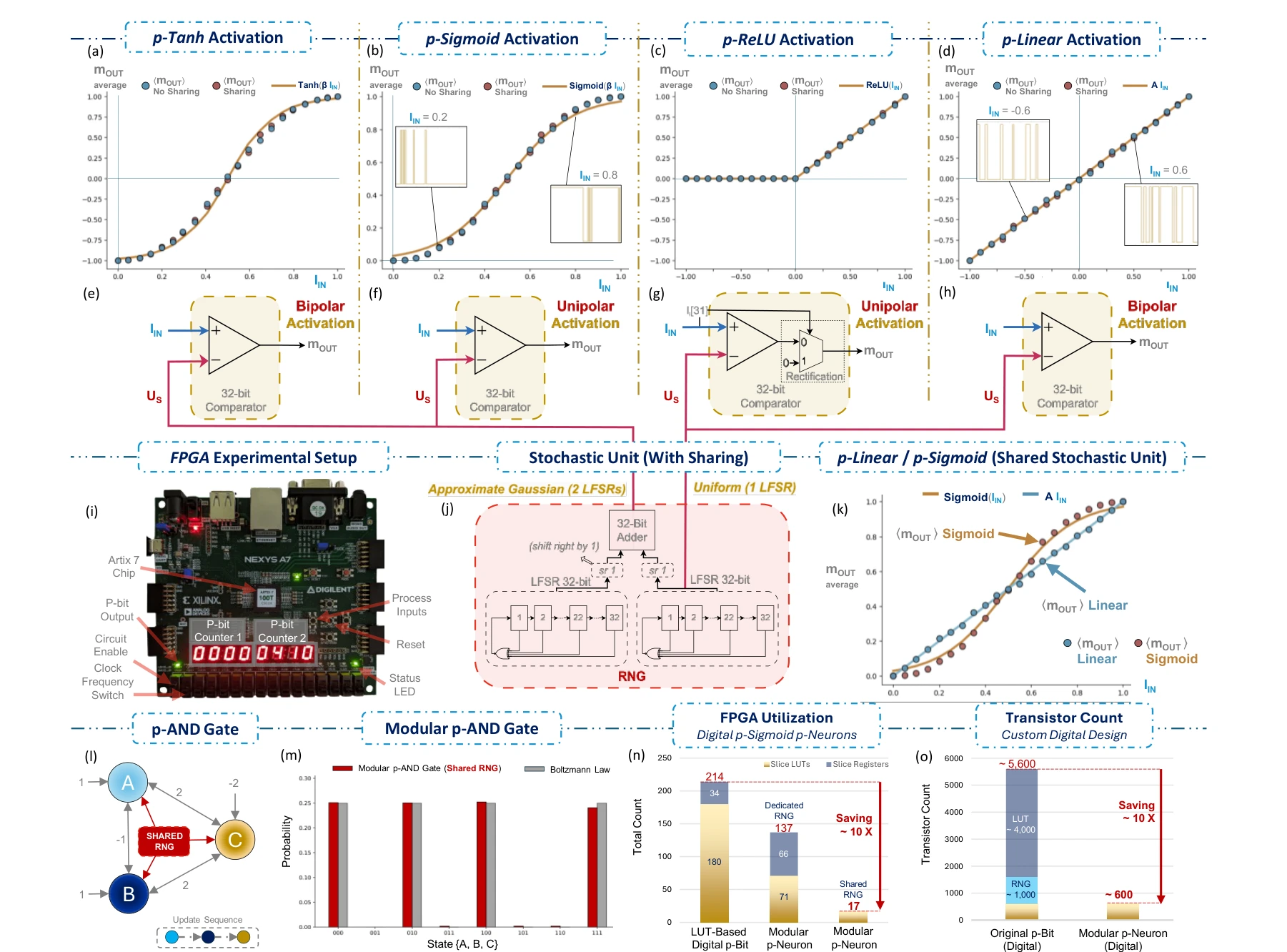
FPGA experiments realize several activation functions and examine stochastic-unit sharing. A small p-AND network checks functional behavior, while resource comparisons show the hardware implications of sharing the random-number source.
Panels (a)–(h). The first four panels show measured average responses for digital tanh, sigmoid, ReLU, and linear neurons. The corresponding designs underneath compare a digital input with a random number supplied by the stochastic unit.
Panels (i)–(m). The hardware photograph and sharing diagrams connect those responses to FPGA experiments. The p-AND example uses three neurons sharing one random-number source; its state histogram is compared with the expected Boltzmann distribution.
Panels (n) and (o). Resource-utilization and transistor-count comparisons quantify the architectural motivation. Read these alongside the sharing experiments: the reduction comes from reusing stochastic resources, while each neuron retains its own activation path.
 Expand figure ↗
Putting it together
Separating the stochastic and activation paths creates configurable building blocks. The digital experiments connect that modularity to functional networks and reduced hardware resource requirements.
Bunaiyan, S., Alsharif, M., Abdelrahman, A. S., ElSawy, H., Cheema, S. S., Fahmy, S. A., Camsari, K. Y., & Al-Dirini, F. Configurable p-Neurons Using Modular p-Bits. IEEE International Symposium on Circuits and Systems (ISCAS) (2026). https://doi.org/10.1109/ISCAS66217.2026.11562319
@inproceedings{bunaiyan2026pneurons,
  title = {Configurable p-Neurons Using Modular p-Bits},
  author = {Bunaiyan, Saleh and Alsharif, Mohammad and Abdelrahman, Abdelrahman S. and ElSawy, Hesham and Cheema, Suraj S. and Fahmy, Suhaib A. and Camsari, Kerem Y. and Al-Dirini, Feras},
  booktitle = {2026 IEEE International Symposium on Circuits and Systems (ISCAS)},
  year = {2026},
  doi = {10.1109/ISCAS66217.2026.11562319}
}
Statistical device models and the behavior of delayed physical systems.
Two identical oscillators share a spring. Change their coupling to see how motion moves between them.
Undamped model without delay.
Time in model units · curves show displacement
Displacement of the two oscillators.
Abdelrahman S. Abdelrahman1, Hesham ElSawy2, Yue Yuan3, Suraj S. Cheema4,5,10, Deji Akinwande6, Mario Lanza7,8,9, Feras Al-Dirini2,10
Making a switching layer thinner does not remove the randomness of its defects. This paper builds a framework from defect statistics upward, then checks device-level predictions and explores what changes at extreme miniaturization. Its figures connect atomic structure to manufacturing-relevant behavior.
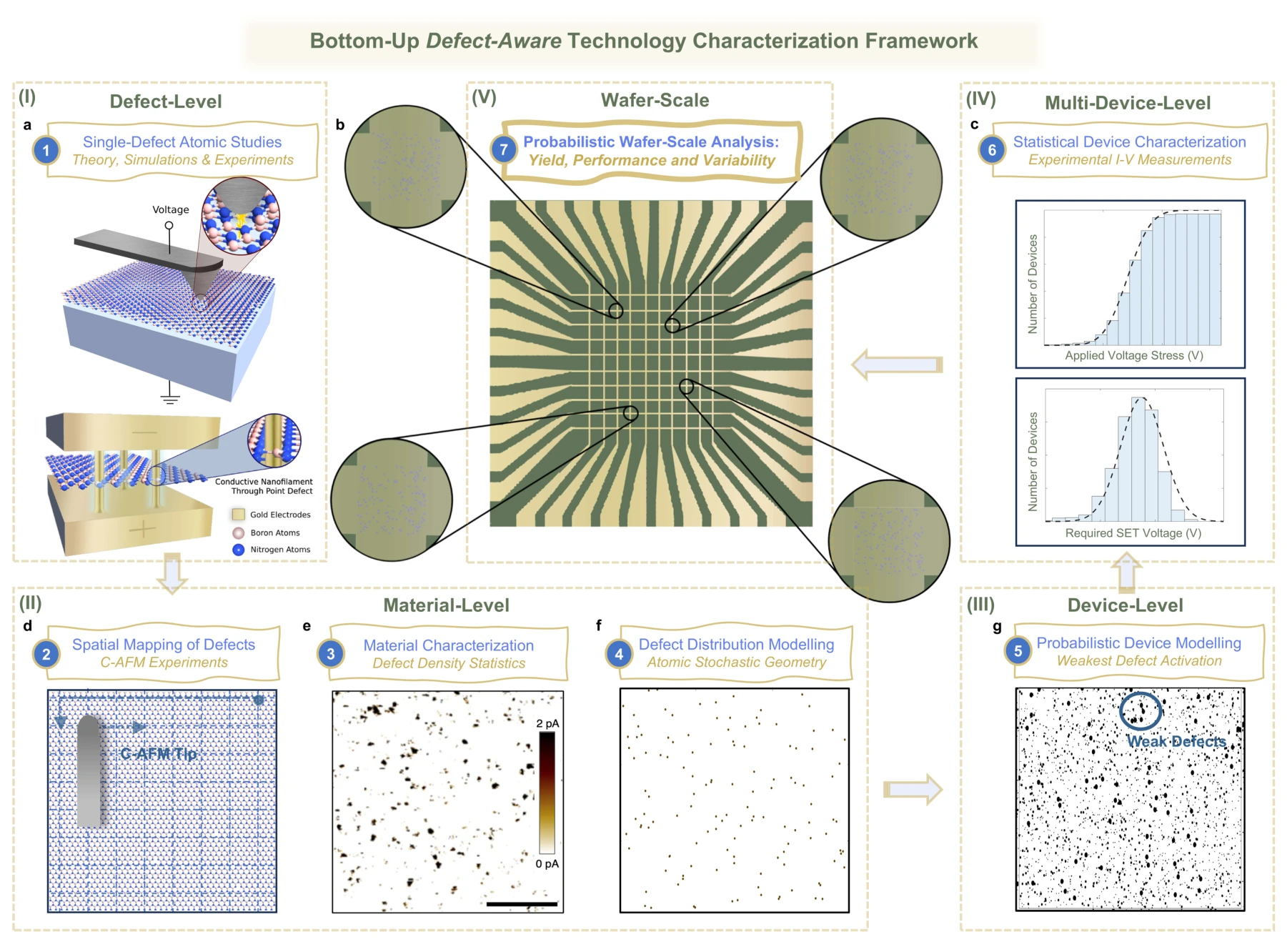
The framework moves through several levels of description: individual defect behavior, spatial material statistics, and the response of a complete device. This organization links microscopic assumptions to quantities such as yield and operating voltage.
Panel (a) and panels (d)–(f). The framework starts with an individual defect and a switching structure, then moves to microscopy and spatial maps of many defects. The material model connects atom-scale information to a statistical description of the film.
Panels (g) and (c). The device model assigns switching behavior to a realization of defects. Measurements across multiple devices then constrain its statistical parameters; the displayed yield data represent a device population, rather than a single switching trace.
Panel (b). The crossbar illustration is the final scale of the framework. Devices within an array can contain different defect realizations, so predictions of yield and variability must carry the underlying stochastic model through to the array level.
 Expand figure ↗
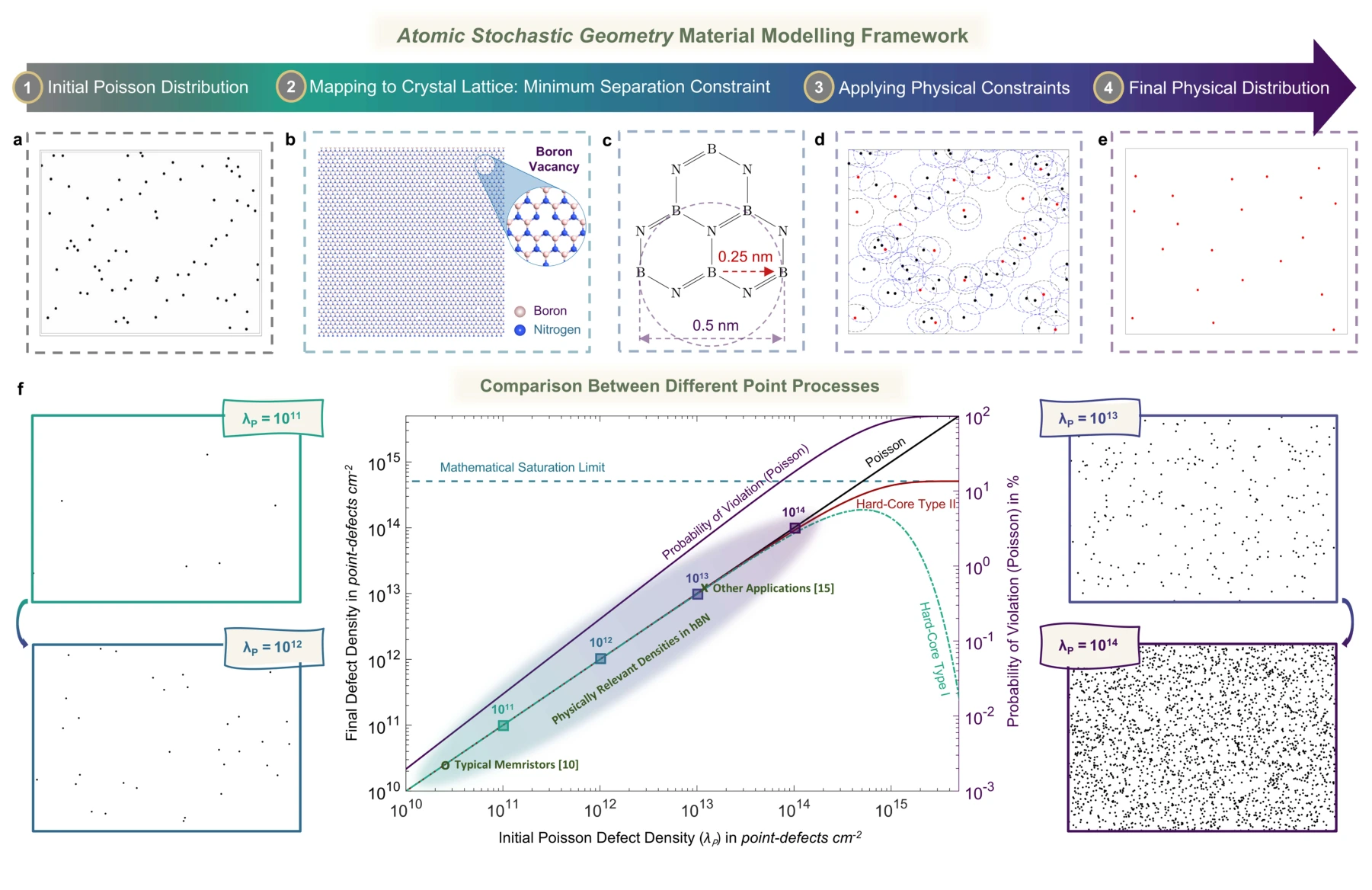
Poisson and hard-core point processes describe different spatial assumptions about defects. Comparing these models shows when exclusion distances matter and how physically constrained defect distributions differ from unconstrained random placement.
Panels (a)–(c). A Poisson point process supplies a starting spatial model, while the h-BN lattice introduces a minimum separation between admissible vacancy locations. An unconstrained random placement need not respect that atomic distance.
Panels (d) and (e). The hard-core construction removes points that violate the separation rule. Black points in the construction are removed; retained red points form the constrained realization shown separately in the next panel.
Panel (f). The density comparison shows how the Poisson and hard-core models diverge as defects become crowded. The saturation bound and constraint-violation probability identify when an unconstrained spatial approximation becomes physically problematic.
 Expand figure ↗
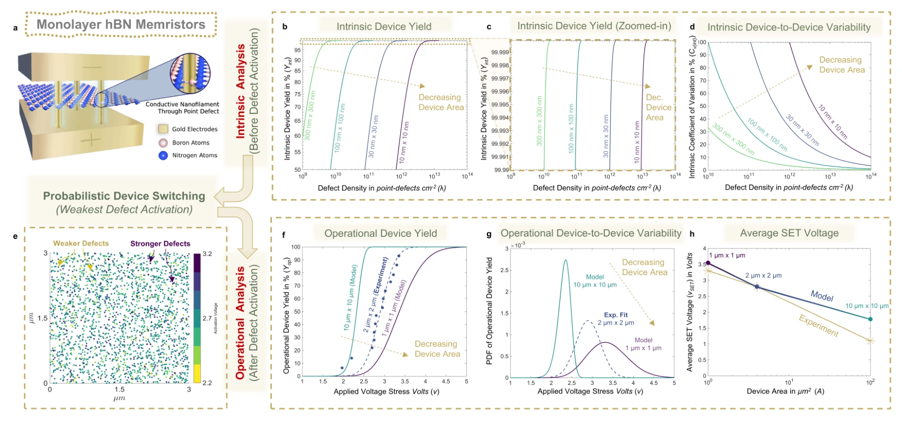
The model connects device area and defect density to intrinsic yield, switching-voltage distributions, and variability in monolayer h-BN memristors. Experimental comparisons provide a check on the statistical predictions.
Panels (a)–(e). The device schematic and defect realization connect the material model to intrinsic yield and variability. Area and defect density control how many potential switching sites a device contains.
Panels (f)–(h). Applied-voltage yield curves become switching-voltage distributions and an area-dependent voltage prediction. Experimental points provide the comparison for the probabilistic device model.
 Expand figure ↗
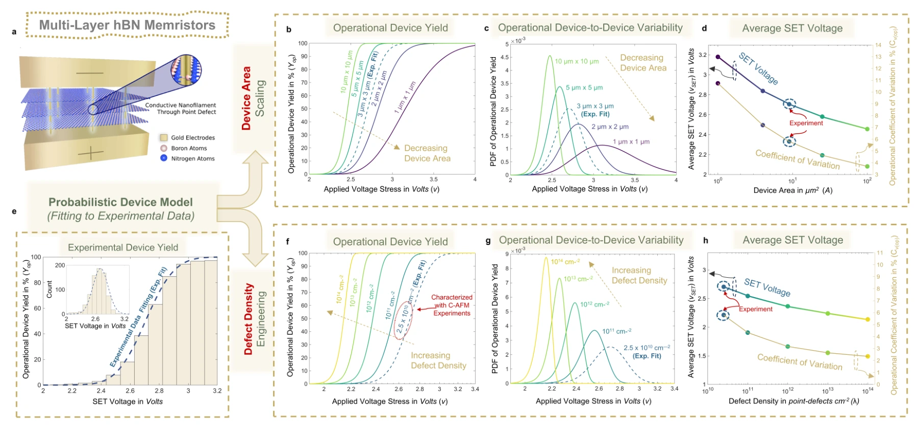
A multilayer switching path changes which defects must participate in conduction. The figure applies the framework to multilayer h-BN devices and compares area-dependent predictions with measured switching behavior.
Panels (a)–(d). The multilayer switching structure is followed by area-dependent yield curves, voltage distributions, and voltage/variability summaries at fixed defect density.
Panels (e)–(h). Measured switching statistics anchor the model. Holding area fixed while changing defect density then separates a material-distribution effect from the device-area sweep above.
 Expand figure ↗
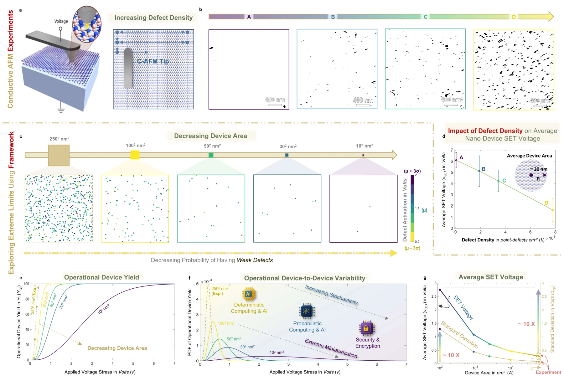
Nanoscale characterization and model extrapolations probe the consequences of reducing device area. The results distinguish a device being able to switch from it doing so with favorable voltage and device-to-device variability.
Panels (a), (b), and (d). Conductive-AFM measurements connect nanoscale switching voltages to films with different measured defect densities. The current maps are thresholded to make individual defects visible; the voltage plot includes experimental variability.
Panel (c). The spatial realizations shrink the device area while marking defects by their activation voltage. Smaller devices contain fewer candidate switching sites, so different defect realizations can lead to different device responses.
Panels (e)–(g). Operational-yield curves are translated into switching-voltage distributions and then into mean voltage and standard deviation. Reading all three separates the chance of switching from the spread of voltages among devices.
 Expand figure ↗
Putting it together
The same defect population influences yield, voltage, and variability in different ways. Evaluating those quantities together makes the tradeoffs of miniaturization more explicit than a dimensional scaling argument alone.
Abdelrahman, A. S., ElSawy, H., Yuan, Y., Cheema, S. S., Akinwande, D., Lanza, M., & Al-Dirini, F. Defect-Aware Extreme Device Scaling Limits of 2D Memristive Technologies. Research Square (2025). https://doi.org/10.21203/rs.3.rs-7265912/v1
@misc{abdelrahman2025defect,
  title = {Defect-Aware Extreme Device Scaling Limits of 2D Memristive Technologies},
  author = {Abdelrahman, Abdelrahman S. and ElSawy, Hesham and Yuan, Yue and Cheema, Suraj S. and Akinwande, Deji and Lanza, Mario and Al-Dirini, Feras},
  year = {2025},
  publisher = {Research Square},
  doi = {10.21203/rs.3.rs-7265912/v1},
  url = {https://www.researchsquare.com/article/rs-7265912/v1}
}
Abdelrahman S. Abdelrahman1, Hesham ElSawy2, Mario Lanza3, Deji Akinwande4, Feras Al-Dirini1,5
How do randomly located defects affect the reliability of an increasingly small memristor? This conference paper begins with a spatial defect model, connects it to measured switching behavior, and follows the consequences of reducing area for monolayer and multilayer devices.
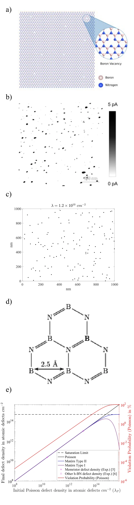
The schematic, microscopy example, and stochastic realization introduce the physical origin of switching sites. The modeling steps connect the distribution of those sites to the probability of obtaining an operational device.
Panels (a) and (b). The defect schematic and conductive-AFM image motivate a spatial model: switching-relevant sites are distributed across the material, rather than guaranteed to appear in the same place in every device.
Panels (c) and (d). The point-process realization is a mathematical representation of those locations. The lattice drawing adds the atomic-scale constraint that neighboring vacancy sites cannot be arbitrarily close together.
Panel (e). The density plot compares the Poisson model with two hard-core processes and a saturation limit. Its second axis tracks the Poisson model’s distance-constraint violations. This explains where a convenient random-placement model needs a physical correction.
 Expand figure ↗
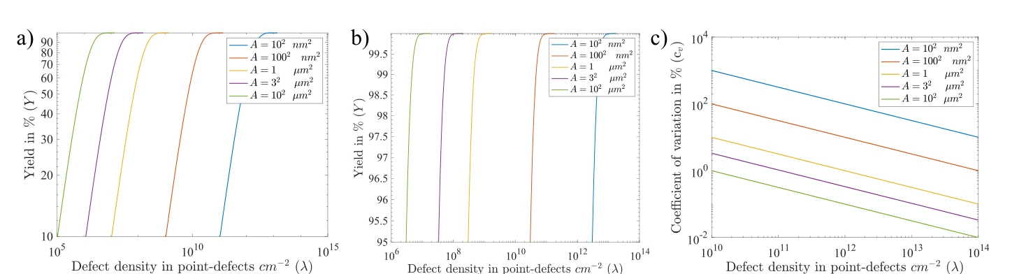
A smaller device contains fewer possible switching sites. These curves show how the intrinsic yield and its variability change with both defect density and device area, including the high-yield regime.
Panels (a)–(c). The yield sweep, high-yield enlargement, and coefficient of variation separate the probability of having defects from variability between device realizations.
 Expand figure ↗
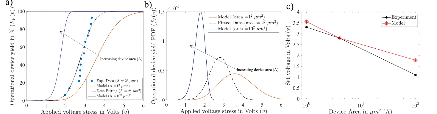
Area-dependent switching-voltage curves are fitted to reported monolayer measurements and then extrapolated. The comparison connects the spatial defect model to an experimentally measurable operating quantity.
Panels (a)–(c). Operational yield is converted into a voltage distribution, then compared with measured switching voltage across device areas. This tests voltage predictions as well as yield.
 Expand figure ↗
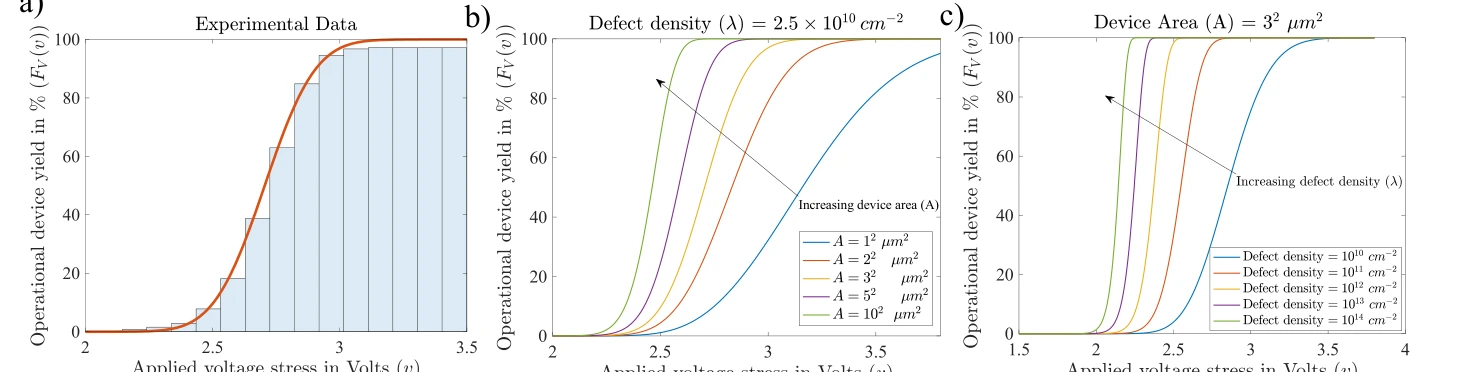
The multilayer case uses measured voltage-dependent yield to calibrate the model. Predicted curves then examine how changes in defect density and device area shift the operational response.
Panels (a)–(c). Measured multilayer-device statistics establish the fit. Subsequent model sweeps change device area and defect density separately to expose their distinct effects.
 Expand figure ↗
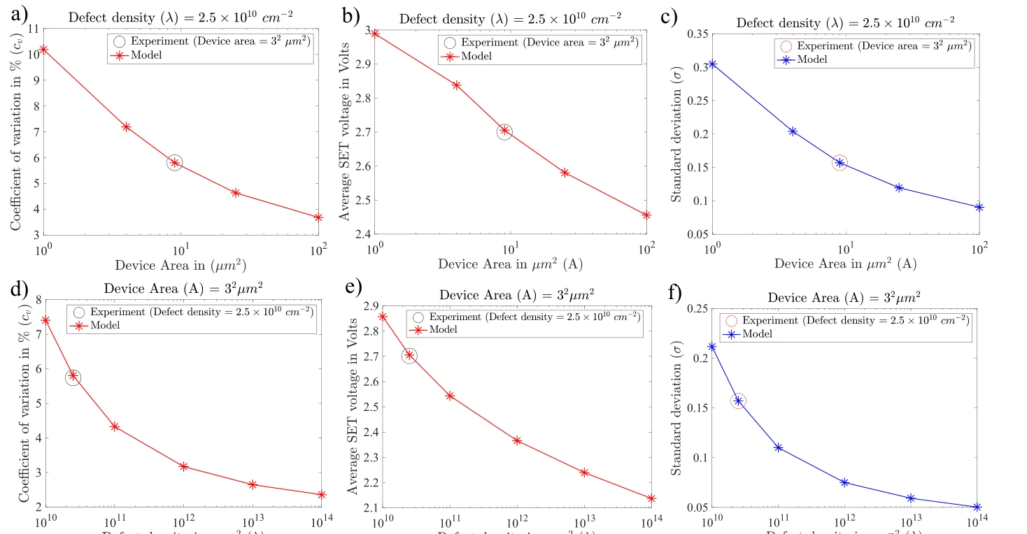
The final panels bring together variation, average SET voltage, and standard deviation across area scales. Reading them together shows why a high switching yield alone is not a complete measure of device quality.
Panels (a)–(c). Coefficient of variation, mean SET voltage, and standard deviation are plotted against device area. The three measures distinguish relative spread from the absolute voltage scale.
Panels (d)–(f). The same quantities are then plotted against defect density at fixed area. Comparing the two rows shows why improving one variability measure cannot be interpreted without the corresponding voltage and geometry.
 Expand figure ↗
Putting it together
The conference study makes yield and variability part of the same scaling problem. The later defect-aware framework develops this direction into a broader bottom-up description.
Abdelrahman, A. S., ElSawy, H., Lanza, M., Akinwande, D., & Al-Dirini, F. Scalability of h-BN Based Memristors: Yield and Variability Considerations. Silicon Nanoelectronics Workshop (2023).
@inproceedings{abdelrahman2023scalability,
  title = {Scalability of h-BN Based Memristors: Yield and Variability Considerations},
  author = {Abdelrahman, Abdelrahman S. and ElSawy, Hesham and Lanza, Mario and Akinwande, Deji and Al-Dirini, Feras},
  booktitle = {2023 Silicon Nanoelectronics Workshop (SNW)},
  year = {2023},
  doi = {10.23919/SNW57900.2023.10183973}
}
Fahhad H. Alharbi1,2, Abdelrahman S. Abdelrahman1, Abdullah M. Alkathiry1, Hussain M. Al-Qahtani3
Two coupled oscillators can exchange energy in ways that resemble a two-level system. Adding a delay changes the mode spectrum and stability of that exchange. The paper follows the connection from a mechanical model through eigenvalue structure to time-domain energy dynamics.
A two-mass spring model establishes the degrees of freedom, damping, and coupling. It provides a classical setting in which the consequences of finite interaction delay can be studied explicitly.
Model components. The masses and wall springs define the uncoupled oscillators; the coupling and damping terms determine how their motion interacts and decays.
 Expand figure ↗
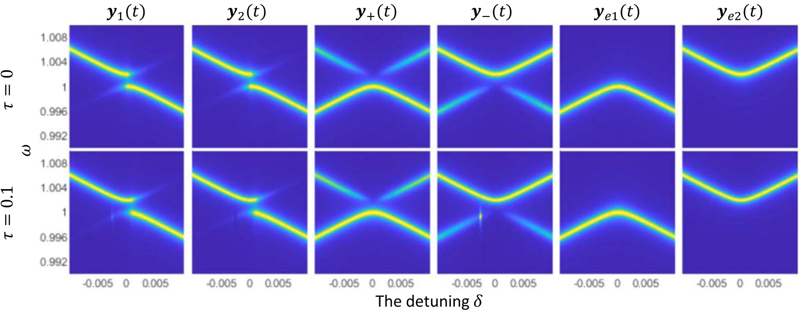
Power spectra for several history functions establish the reference response. Detuning changes which modes are excited and how their resonances appear in the total spectral density.
Upper and lower panels. The upper spectra use zero delay; the lower spectra use a delay of 0.1. Different history functions excite different mode combinations, so comparing rows separates delay effects from the initial preparation.
 Expand figure ↗
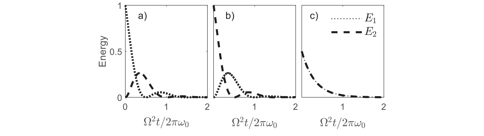
The oscillator energies are plotted for different initial histories. These time-domain examples show how the chosen preparation changes the visible exchange between the two subsystems.
Panels (a)–(c). Three history functions prepare the same coupled system differently. Following both energy curves shows how the preparation changes the observed exchange without changing the model parameters.
 Expand figure ↗
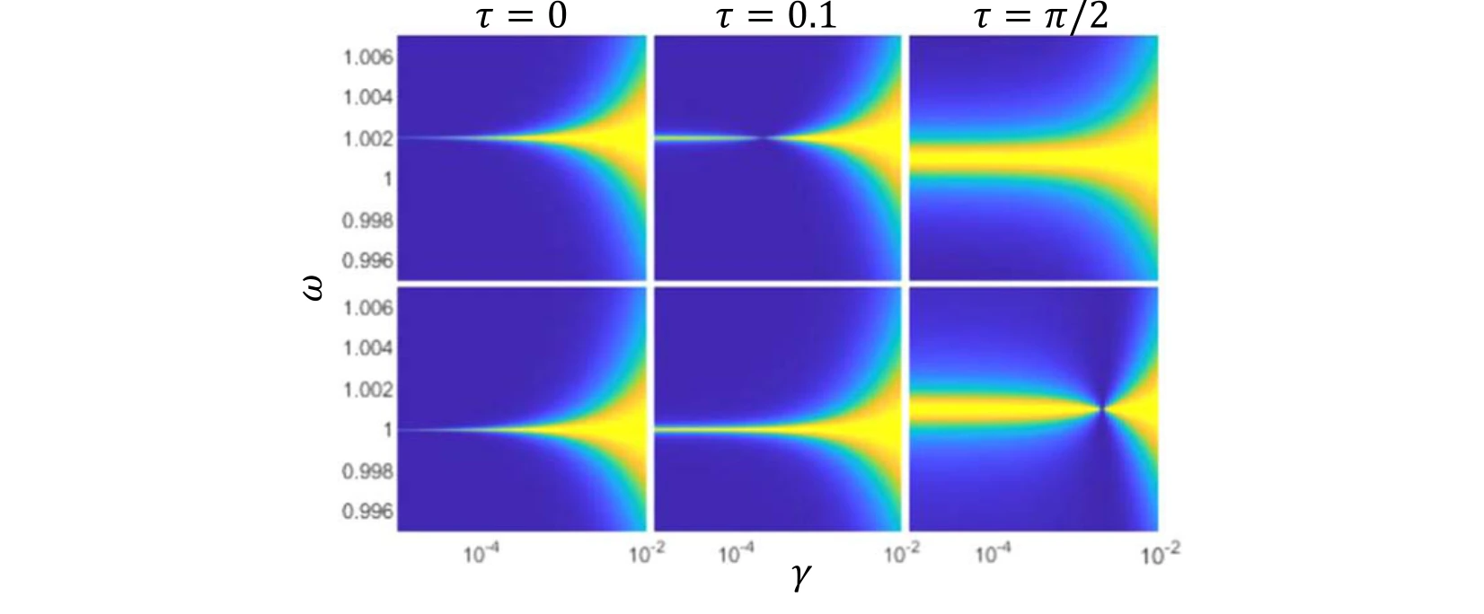
Linewidths of the coupled modes are compared across damping rates and delays. This connects the spectral response to the persistence of the oscillations.
Upper and lower panels. The upper plots follow the second eigenstate and the lower plots the first. Comparing delays at the same damping rate reveals changes in spectral linewidth.
 Expand figure ↗
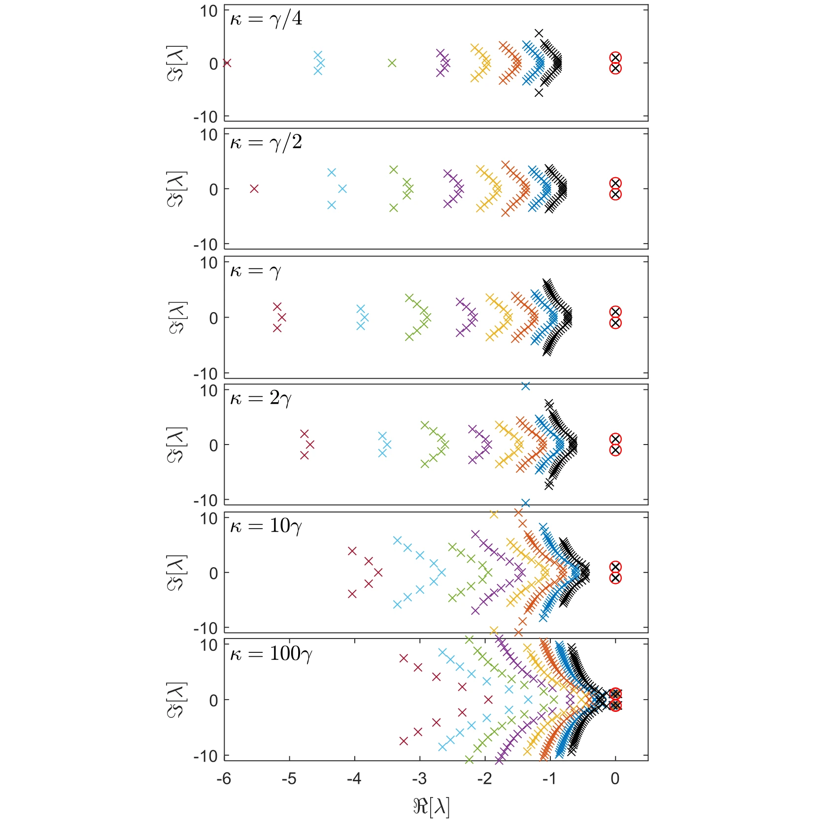
The complex spectrum is plotted for different couplings and delays. Moving beyond the instantaneous model reveals additional structure in the possible dynamical modes.
Across the six rows. The coupling increases from one quarter of the damping rate to one hundred times that rate. Within each row, colors distinguish delays from 0.3 to 1.0, allowing the displacement of the spectrum to be separated from a change in coupling.
The red circles. The two highlighted roots are the main dynamical modes followed in the later figures. Their horizontal position gives the growth or decay rate, while their vertical position gives the oscillation frequency.
Reading the comparison. Use the same axes to compare the circled pair with the other roots. The figure establishes which part of the spectrum is being tracked before subsequent plots focus on the dominant pair and the stability boundary.
 Expand figure ↗
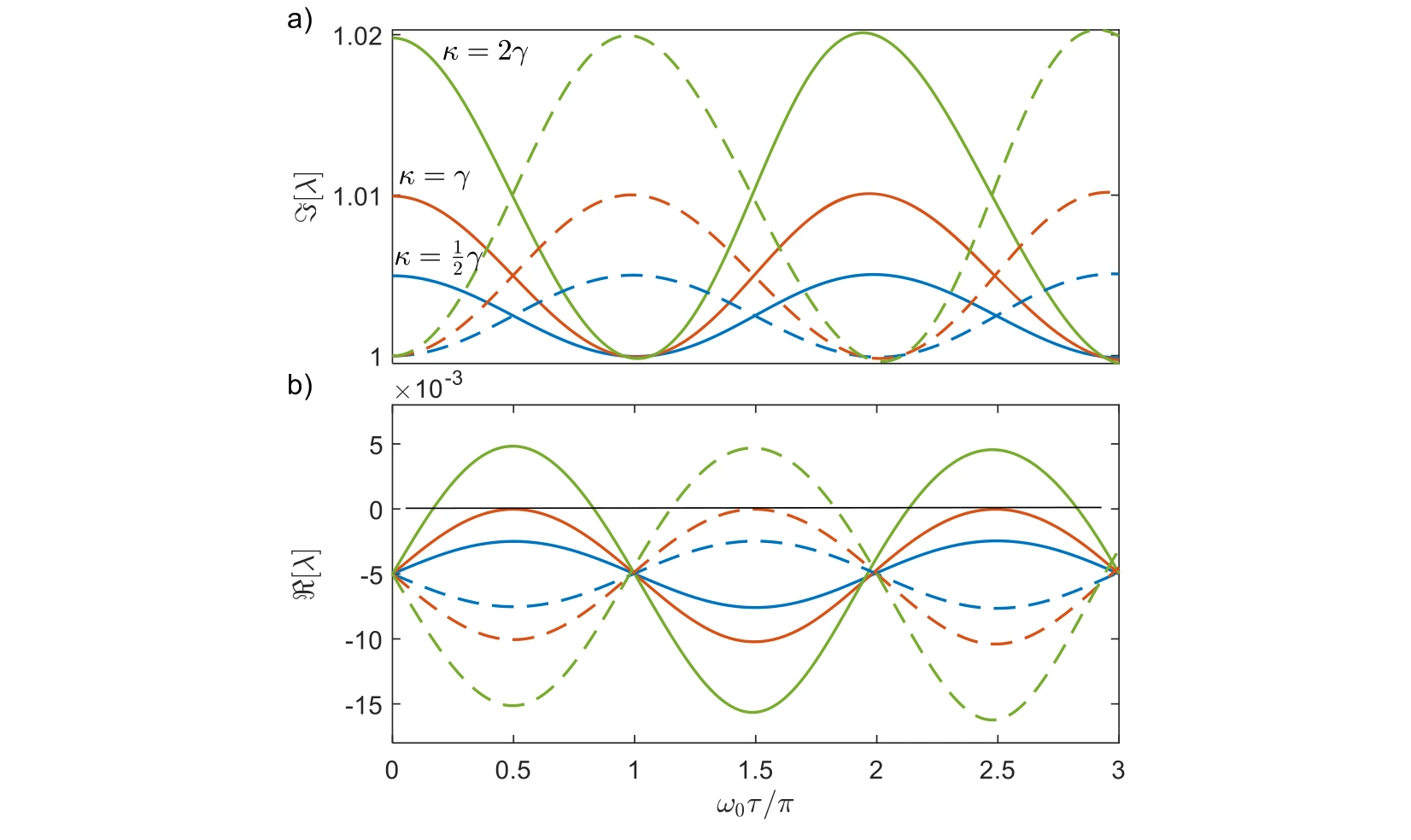
Real and imaginary parts of the main modes are followed across delay. Their trajectories distinguish changes in oscillation frequency from changes in stability or decay.
Real and imaginary components. The two plots separate changes in decay or growth from changes in oscillation frequency. Solid and dashed curves of the same color identify the two main modes at a fixed coupling.
The stability boundary. The black zero-real-part line marks the transition between decay and growth. Comparing the three coupling choices—half, equal to, and twice the damping rate—shows why frequency splitting alone does not establish stable dynamics.
 Expand figure ↗
The rightmost eigenvalues determine whether a mode grows or decays most slowly. Comparing coupling strengths exposes how the dominant dynamical behavior changes with delay.
Top row. The imaginary parts track oscillation frequencies as normalized delay changes. Following both branches reveals how the dominant pair evolves across the tested coupling strengths.
Middle and bottom rows. Positive real parts are plotted separately from negative real parts. That separation makes unstable growth distinguishable from damped motion, even when their frequency branches look similar.
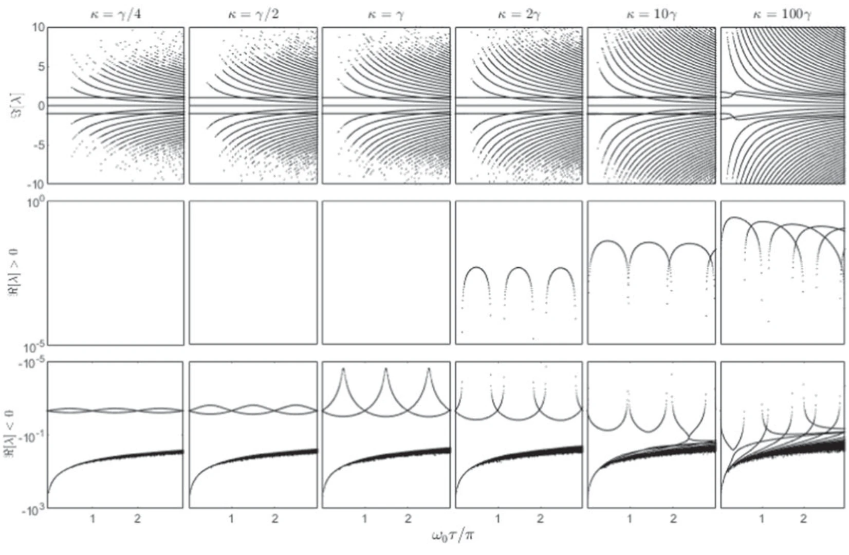 Expand figure ↗
The eigenvalue paths offer another representation of the same delayed dynamics. Their geometry clarifies how conjugate modes move as the interaction delay varies.
Panels (a) and (b). These trajectories follow the upper pair of coupled modes in the complex plane. Read horizontal displacement as a change in the real part and vertical displacement as a change in frequency.
Panels (c) and (d). The lower panels show the corresponding conjugate modes. Viewing the pairs together links the separate real- and imaginary-part plots to complete eigenvalue trajectories as delay varies.
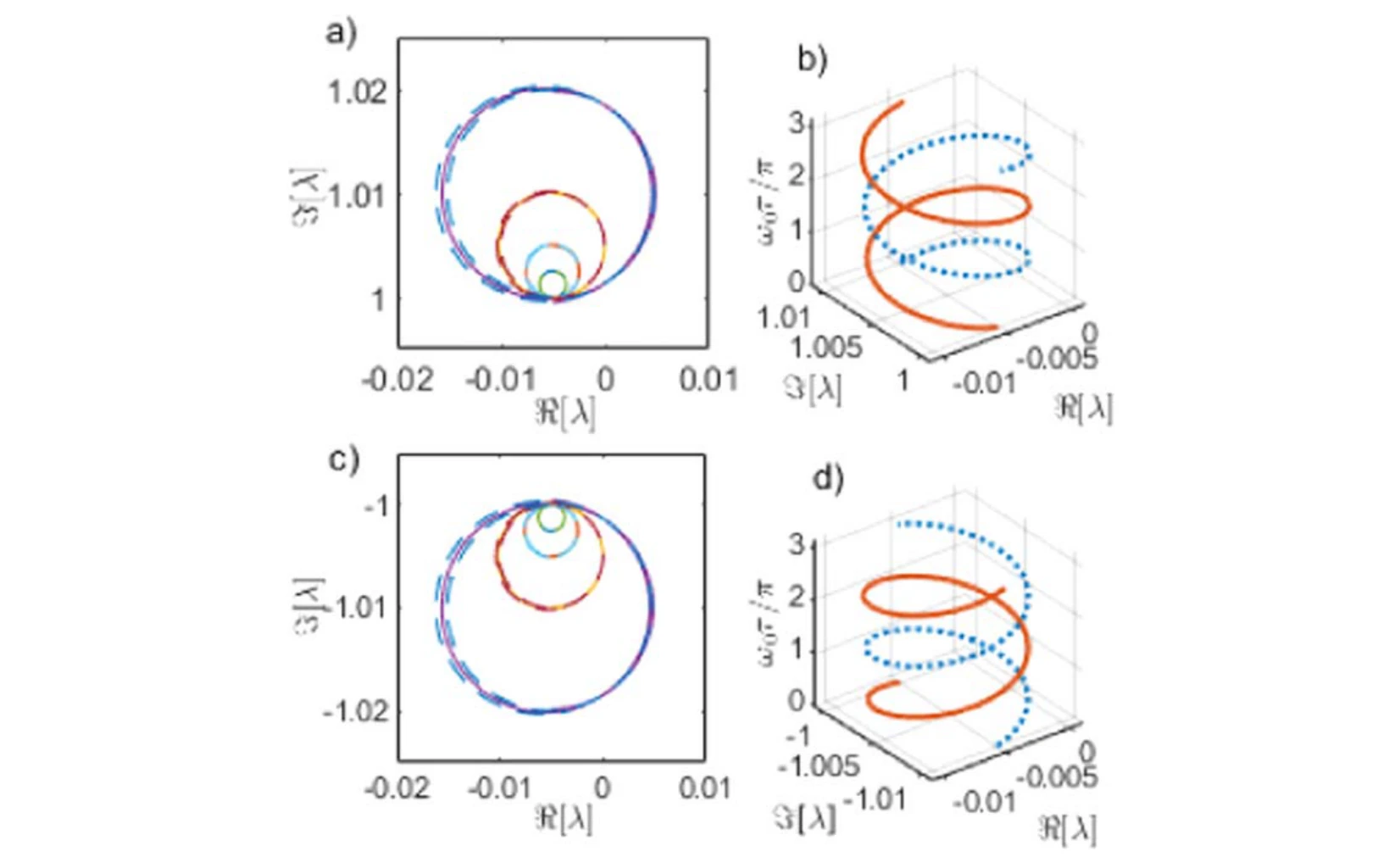 Expand figure ↗
A schematic condenses the evolution into circles and interwinding trajectories. It provides a visual guide to the more detailed eigenvalue plots that precede it.
Reading the schematic. The circles summarize the mode paths in the preceding complex-plane plots. Their overlap and interwinding organize the recurring evolution with delay; the drawing is a geometric guide to those trajectories, rather than another time-domain measurement.
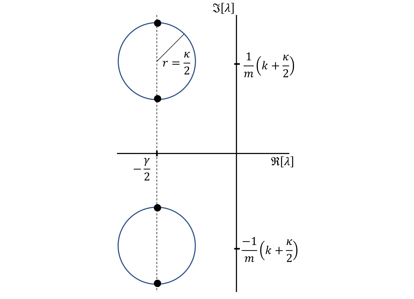 Expand figure ↗
The stability map gathers intervals in which eigenvalues imply growing motion. Comparing different coupling strengths shows how stable and unstable delay ranges alternate.
Stable intervals. Gray intervals in the upper panel mark stable dynamics. Comparing their widths and locations as coupling increases makes the repeated stable and unstable delay regions easier to identify than in individual root plots.
Connection to the spectrum. These intervals summarize where the leading eigenvalues have the sign required for decay. They should be read together with the real-part plots, which show how a mode reaches the stability boundary.
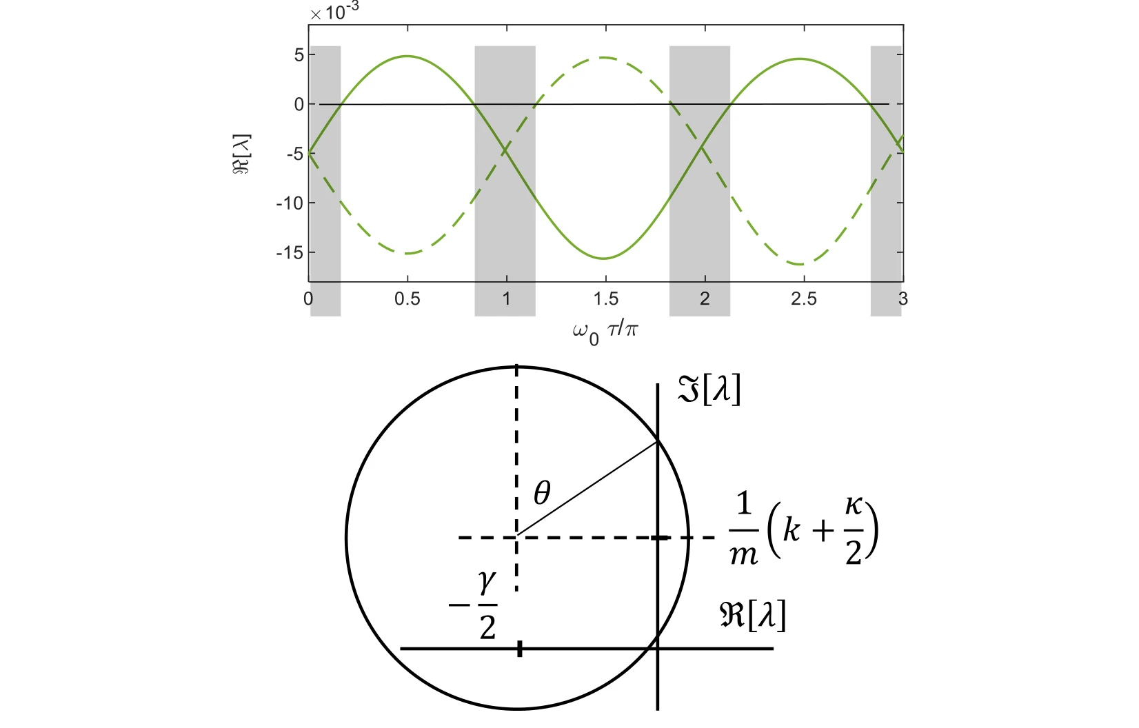 Expand figure ↗
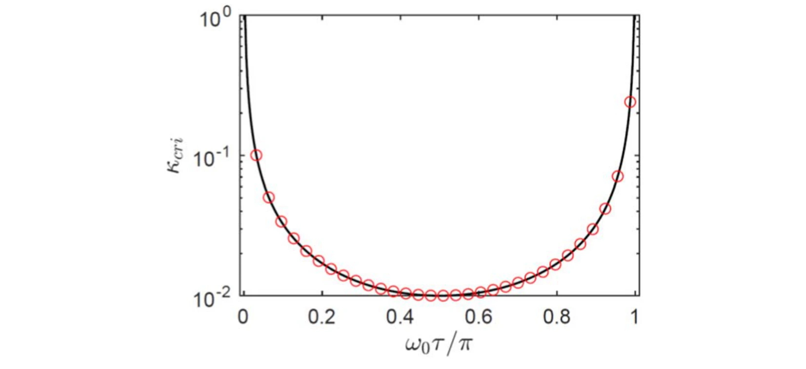
A bifurcation diagram plots the critical coupling against normalized delay. It connects the observed stability transitions with the boundary predicted by the dynamical analysis.
Curve and markers. The black bifurcation boundary plots critical coupling against normalized delay. Red circles evaluate the derived stability condition, providing a direct check against that boundary.
 Expand figure ↗
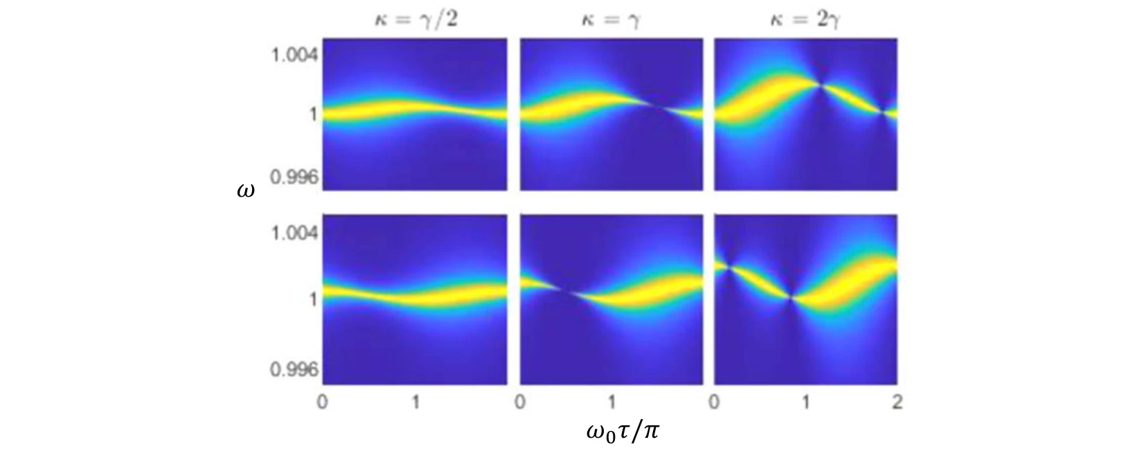
Power-density plots compare several coupling cases and history functions as delay varies. They connect changes in the eigenvalue picture to observable spectral features.
Rows and columns. The rows correspond to the two eigenstates. The three coupling choices—half, equal to, and twice the damping rate—show how the delay-dependent spectra change across the coupling boundary.
 Expand figure ↗
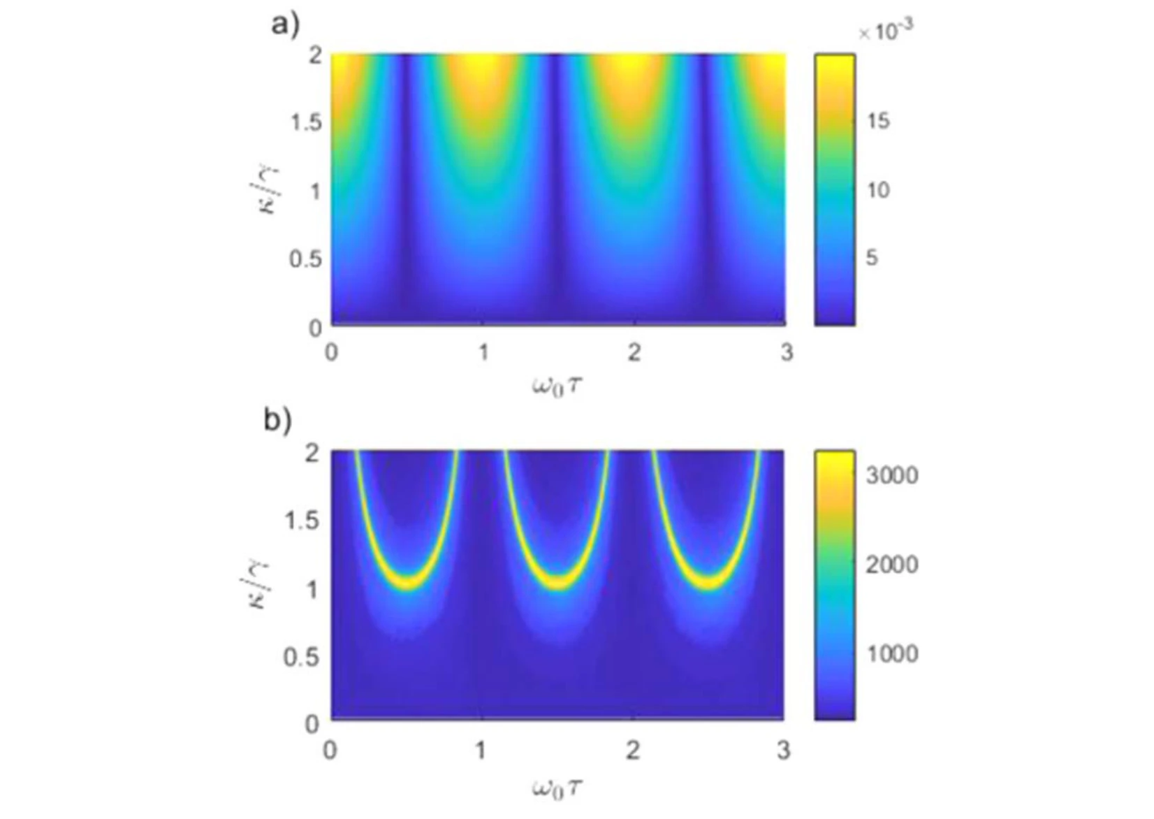
The exchange frequency and coherence time are mapped across coupling and delay. These quantities summarize how quickly energy moves and how long the exchange remains discernible.
Panel (a). The energy-exchange frequency is plotted against both coupling and delay. It describes how quickly energy moves between the oscillators; it is a different quantity from the individual oscillators’ carrier frequencies.
Panel (b). The coherence-time surface measures how long the exchange remains coherent under the same parameter variation. Comparing the surfaces separates a faster transfer process from a longer-lived one.
 Expand figure ↗
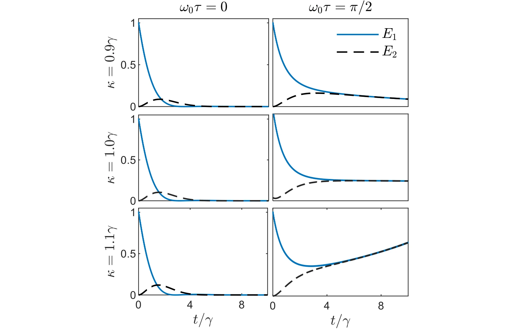
Time traces compare the individual oscillator energies for couplings around the damping scale. The cases place the abstract coherence and stability measures back into direct energy dynamics.
Across the rows. The coupling is 0.9, 1.0, and 1.1 times the damping rate. These closely spaced choices probe the region around the coupling boundary instead of comparing only widely separated regimes.
Across the columns. The left and right columns use normalized delays of zero and π/2. Each plot follows both oscillator energies, making the effect of delay visible at the same coupling.
 Expand figure ↗
The final trajectories broaden the coupling comparison and contrast instantaneous with delayed interaction. They complete the connection between the spectrum, stability, and the observed energy exchange.
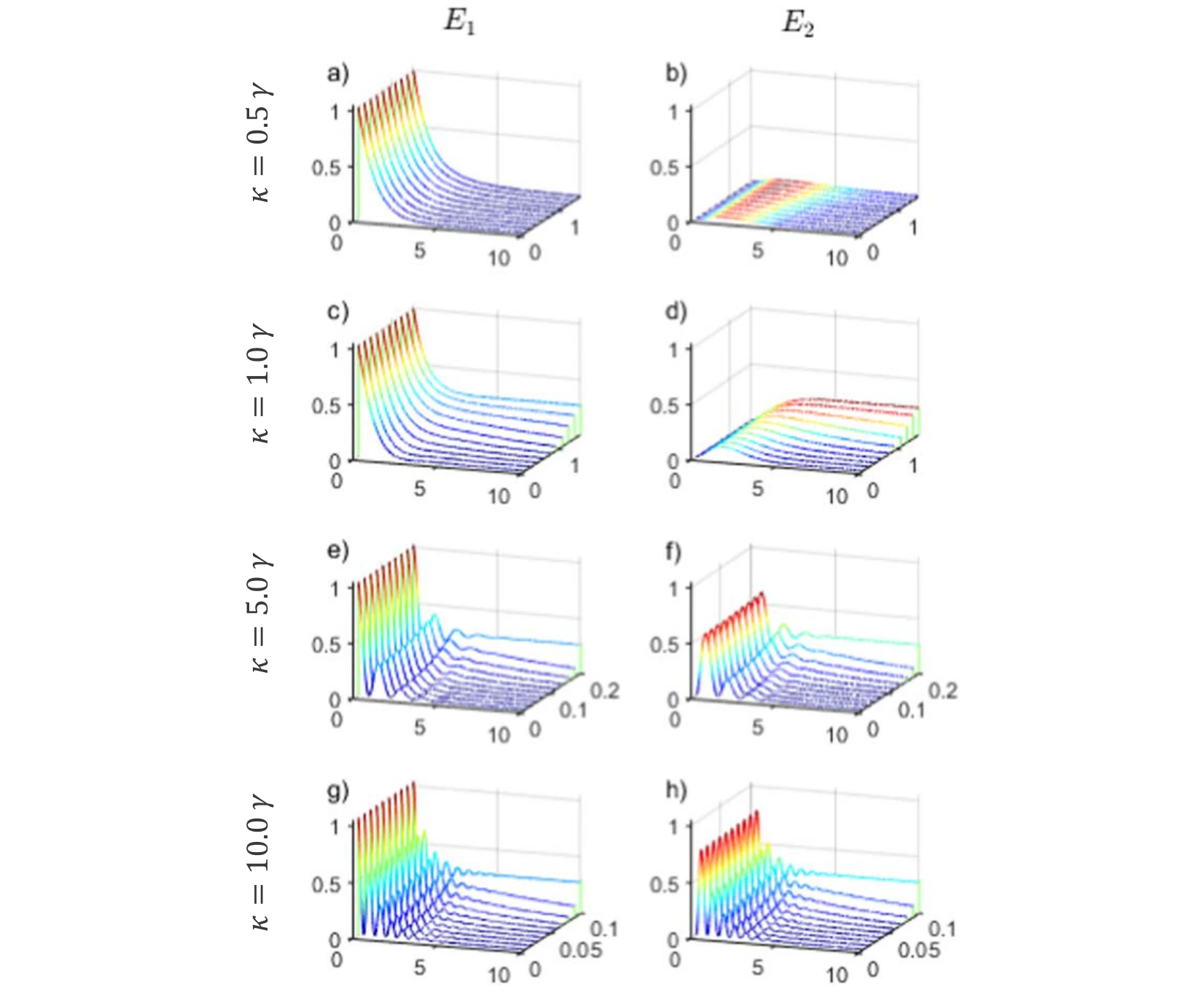
Panels (a), (c), (e), and (g). The left column shows the first oscillator’s energy. From top to bottom, coupling rises from 0.5 to 1, 5, and 10 times the damping rate, while each surface varies time and delay.
Panels (b), (d), (f), and (h). The right column follows the second oscillator under the matching conditions. Compare each row as a pair to see transferred energy alongside the energy remaining in the first oscillator.
Reading the surfaces. The oscillatory exchange becomes more apparent in the stronger-coupling rows. The plotted delay range also changes between rows, so matching the axes matters when comparing the extent and persistence of the oscillations.
 Expand figure ↗
Putting it together
Spectra, eigenvalues, stability maps, and energy trajectories describe complementary aspects of the same system. Delay links these views by changing both the allowed modes and the coherence of their energy exchange.
Alharbi, F. H., Abdelrahman, A. S., Alkathiry, A. M., & Al-Qahtani, H. M. Energy Transfer and Coherence in Coupled Oscillators with Delayed Coupling: A Classical Picture of Two-Level Systems. Physica Scripta, 97(8) (2022).
@article{alharbi2022energy,
  title = {Energy transfer and coherence in coupled oscillators with delayed coupling: a classical picture of two-level systems},
  author = {Alharbi, Fahhad H. and Abdelrahman, Abdelrahman S. and Alkathiry, Abdullah M. and Al-Qahtani, Hussain M.},
  journal = {Physica Scripta},
  volume = {97},
  number = {8},
  pages = {085215},
  year = {2022},
  doi = {10.1088/1402-4896/ac7f62}
}
Abdelrahman S. Abdelrahman1, Hussain Al-Qahtani2, Fahhad H. Alharbi1,3
Delayed interactions turn a familiar oscillator problem into a transcendental eigenvalue problem. This study compares four approximation strategies against a shared physical model, separating their predictions for the real and imaginary parts of the fundamental eigenfrequencies.
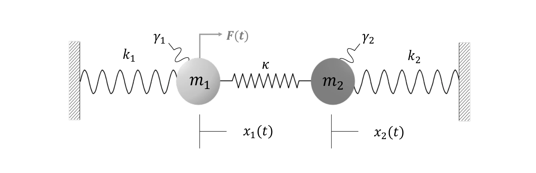
Two coupled mass–spring oscillators provide the common test system. A delay in the interaction changes the characteristic equation, making the calculation of dynamical eigenvalues more demanding than in the instantaneous case.
The common benchmark. The wall springs, masses, and coupling define one mechanical system for every solver. An external force acts on the first mass to initiate the response.
 Expand figure ↗
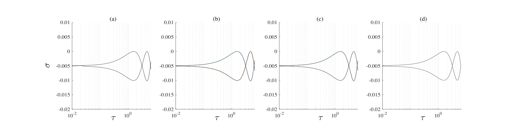
Taylor expansion, Rekasius substitution, self-consistent iteration, and Chebyshev discretization are evaluated as the delay varies. The real components reveal the predicted growth or decay behavior and where the approximations diverge.
Panels (a)–(d). Taylor expansion, Rekasius substitution, self-consistent iteration, and Krylov approximation are applied to the same delay-dependent real components.
 Expand figure ↗
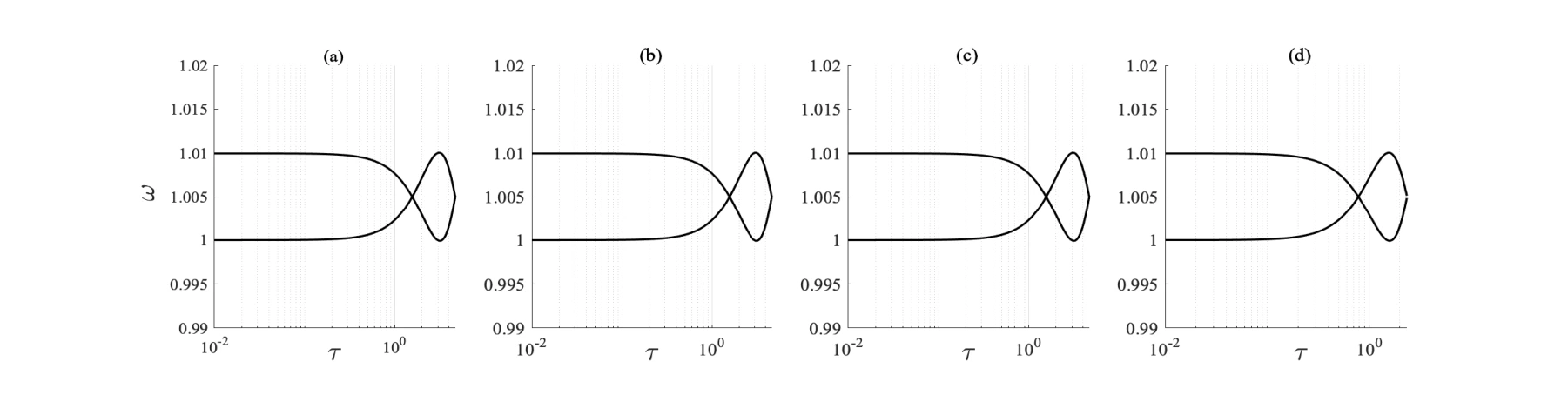
The corresponding imaginary components describe the oscillatory part of the modes. Viewing them alongside the real components exposes differences between methods that a single stability metric could miss.
Panels (a)–(d). The same method order is retained for the imaginary components, allowing each solver’s frequency branches to be read alongside its real-part result.
 Expand figure ↗
Putting it together
Using the same oscillator model makes the numerical methods directly comparable. Real and imaginary eigenvalue components provide complementary checks on the behavior predicted by each approximation.
Abdelrahman, A. S., Al-Qahtani, H. M., & Alharbi, F. H. A Comparison of Numerical Solvers for the Delay Eigenvalue Problem of Coupled Oscillators. Journal of Physics: Conference Series, 1730(1) (2021).
@article{abdelrahman2021delay,
  title = {A Comparison of Numerical Solvers for the Delay Eigenvalue Problem of Coupled Oscillators},
  author = {Abdelrahman, Abdelrahman S. and Al-Qahtani, Hussain and Alharbi, Fahhad H.},
  journal = {Journal of Physics: Conference Series},
  volume = {1730},
  number = {1},
  pages = {012114},
  year = {2021},
  doi = {10.1088/1742-6596/1730/1/012114}
}
Energy-efficient data collection and adaptive statistical estimation.
Omar Khalifa1, Anas S. Mohammed2, Ali Alhejab1, Abdelrahman S. Abdelrahman3, Ahmed Al-Radhwan4, Ruslan Zhagypar1, Hesham ElSawy5, Nour Kouzayha1, Noha Al-Harthi6, Jaafar Elmirghani6, Zekeriya Aksoy6, Tareq Y. Al-Naffouri1
Keeping remote sensors awake wastes energy, but sleeping through a UAV visit loses data. This study develops an addressed wake-up-radio system, validates the hardware, and then connects the prototype to models of timing, reliability, and deployment at network scale.
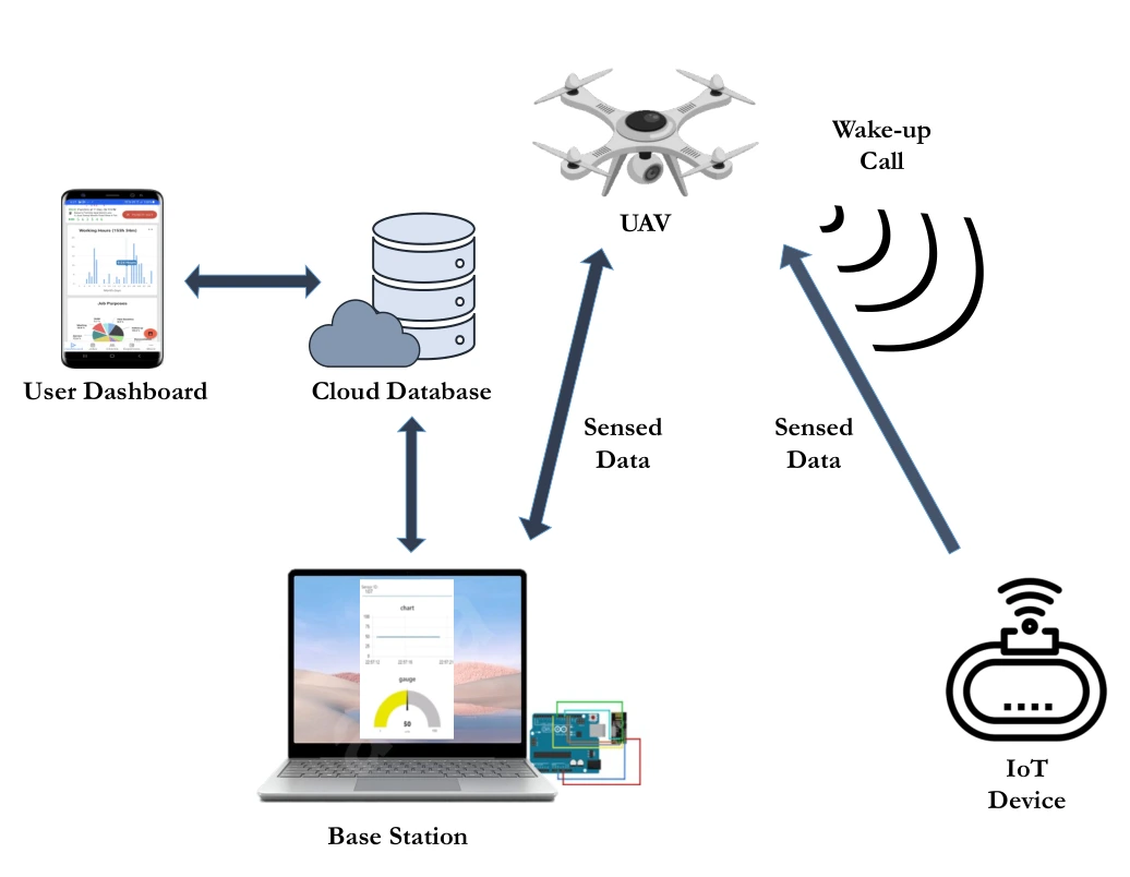
The architecture connects the UAV wake-up transmitter, sleeping IoT node, base station, database, and dashboard. It establishes the path that later hardware and analytical results must support.
Wake-up and data paths. The wake-up call travels from the UAV to the ground device; the sensed data travels back toward the UAV and base station. These arrows separate the low-power activation mechanism from the main data-transfer link.
Ground infrastructure. The base station organizes the collected measurements and uploads them to a cloud database. The dashboard completes the path to the user, making the figure an end-to-end system diagram rather than only a radio-link sketch.
 Expand figure ↗
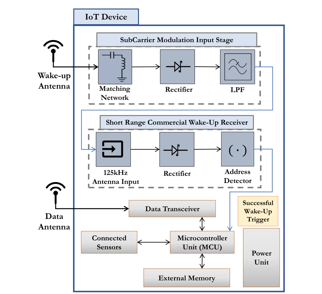
The block diagram separates wake-up detection, addressing, sensing, and data transmission. A successful wake-up event activates the functions that would otherwise consume power while the node waits.
Upper signal path. The subcarrier-modulation input stage contains matching, rectification, and filtering blocks before the commercial wake-up receiver. The receiver then detects an address and issues the wake-up signal.
Lower device blocks. The microcontroller, sensors, memory, and data transceiver perform the sensing and reporting task after activation. Separating these functions explains how the wake-up path can remain available while more power-hungry circuitry sleeps.
 Expand figure ↗
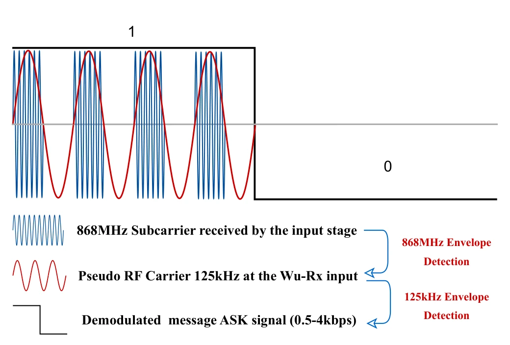
Subcarrier modulation lets a higher-frequency transmitted signal deliver the lower-frequency pattern expected by the wake-up receiver. The waveform connects the radio carrier to the decoded binary message.
Carrier and envelopes. The drawing starts with an 868 MHz subcarrier and shows the lower-frequency envelope recovered from it. A subsequent detection stage exposes the on–off keyed message used by the wake-up receiver.
Reading the bit sequence. Compare the high-frequency oscillations with the slower binary envelope above them. The receiver needs the address-bearing message, rather than the original radio-frequency waveform, which motivates the passive input-stage demodulation.
 Expand figure ↗
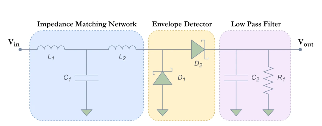
Matching, envelope detection, and low-pass filtering translate the received signal into a form the wake-up receiver can use. The schematic makes the signal-processing path explicit.
Three circuit stages. The matching network couples the antenna to the input; the envelope detector rectifies the signal; the low-pass filter retains the lower-frequency carrier needed by the wake-up receiver.
 Expand figure ↗
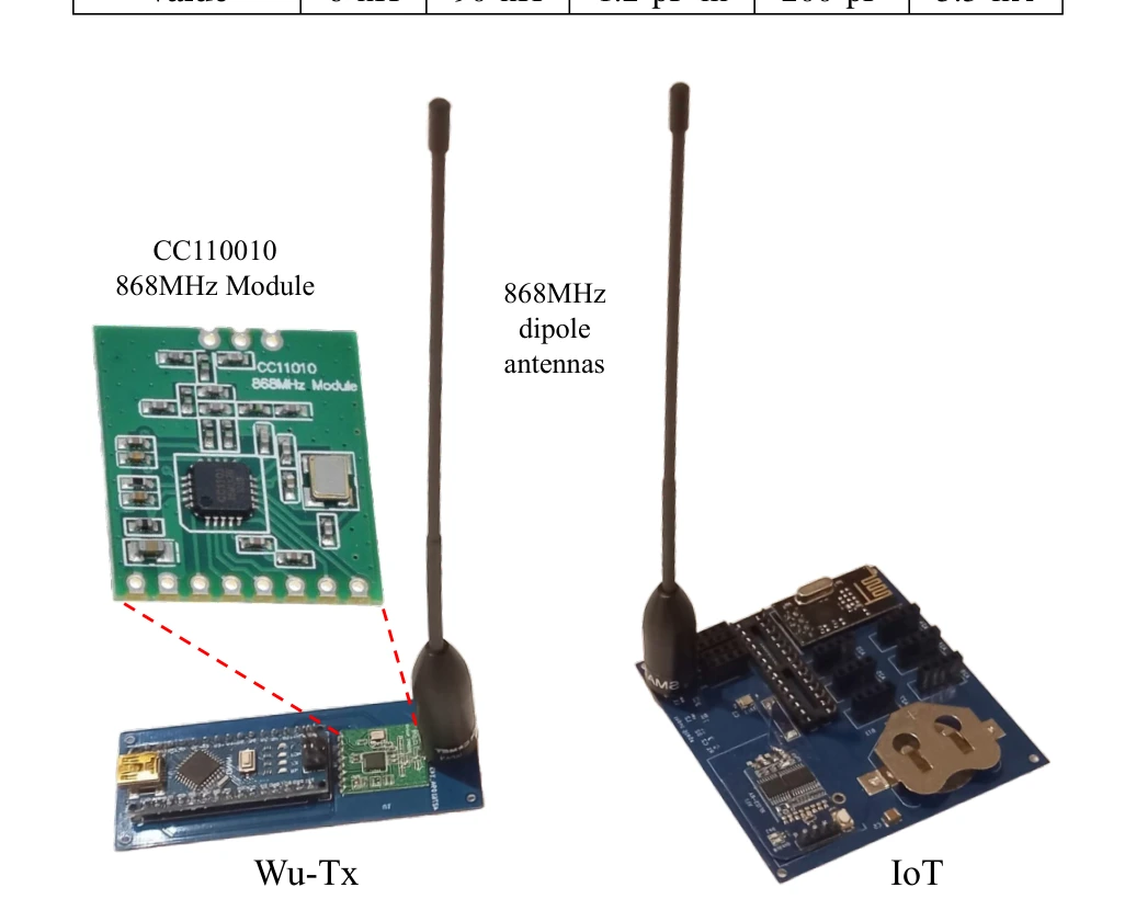
Photographs show the developed IoT device and wake-up transmitter. This step turns the earlier architecture and circuit descriptions into physical components for testing.
The transmitter. The CC1101-based wake-up transmitter and its dipole antenna implement the radio side of the wake-up call. The IoT board provides the corresponding receiver-side hardware, connecting the earlier block diagrams to assembled components.
Why both boards matter. An operational wake-up link depends on the transmitter waveform, antenna, input stage, and receiver together. The photograph documents the prototype used for the following bench, indoor, and aerial experiments; it is not a chip-level integration claim.
 Expand figure ↗
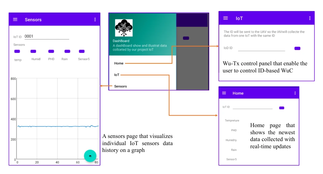
The mobile interface presents sensed data and system controls. It provides the user-facing endpoint of the otherwise hardware-centered data-collection pipeline.
Sensor view. The sensor screen displays collected measurements, completing the path from the ground node through the UAV and base station to the user.
Control and home views. The IoT control screen supports addressed wake-up requests. The remaining view provides navigation among the application’s functions, making the dashboard part of the operational system rather than only a results display.
 Expand figure ↗
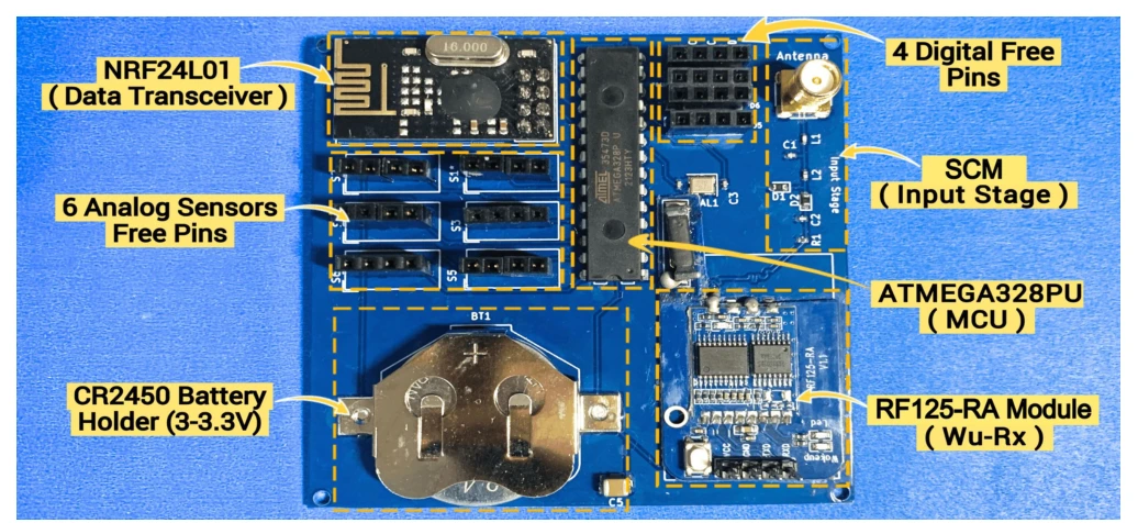
The annotated prototype identifies the microcontroller, sensor interfaces, wake-up module, power source, and data radio. The layout shows how the required functions fit on the actual device.
Hardware integration. The photograph identifies the data transceiver, microcontroller, wake-up receiver, input stage, battery holder, and free sensor pins. Their placement documents how the low-power wake-up path is integrated with a functioning sensing node.
 Expand figure ↗
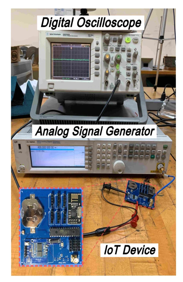
The laboratory setup uses a signal generator and oscilloscope to test subcarrier modulation with the IoT node. This isolates the receive path before outdoor deployment.
Signal source. The microwave signal generator supplies a carrier swept around the intended 868 MHz operating frequency. This isolates the subcarrier-modulation input stage before the complete wake-up protocol is tested.
Measurement. The oscilloscope observes the receiver input-stage output. With a continuous carrier and no slower modulation envelope, rectification and low-pass filtering produce an approximately DC output, so the test checks the input stage’s frequency response.
Scope of this test. This is a bench characterization of the signal-conditioning path. The separate indoor and aerial experiments are needed to establish how the complete wake-up link behaves over distance.
 Expand figure ↗
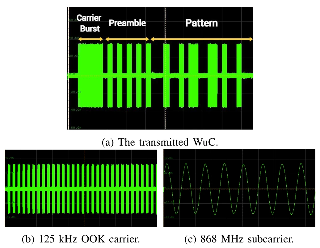
Oscilloscope traces expose the carrier burst, preamble, and address pattern. These measurements check that the transmitted signal contains the structure expected by the receiver.
Panel (a). The complete transmitted wake-up call contains the carrier burst, preamble, and address pattern. Reading these in order shows how a receiver is prepared and then given an identification-bearing message.
Panels (b) and (c). The lower panels zoom into the 125 kHz on–off keyed carrier and the 868 MHz subcarrier. They are different time scales of the same transmitted waveform, rather than two independent communication experiments.
 Expand figure ↗
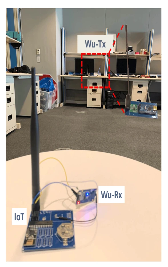
The indoor range experiment tests the transmitter and receiving node in a controlled environment. It provides a practical reference before moving to the aerial configuration.
Test arrangement. The wake-up transmitter is placed across the room from the assembled IoT device and its receiver. This checks the complete link after the input stage has been characterized on the bench.
What changes between tests. The indoor experiment changes separation between the transmitter and receiver. It precedes the aerial test, where antenna alignment and UAV motion introduce additional conditions that a room-scale stationary setup does not capture.
Reading the photograph. The labeled receiver is part of the powered IoT prototype. Successful wake-up refers to activating that device through the wake-up path, not merely observing an RF signal at an instrument input.
 Expand figure ↗
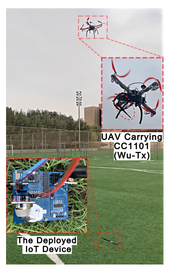
The outdoor setup combines a flying transmitter with the deployed IoT node. It tests the intended data-collection geometry rather than a fixed bench arrangement.
On the UAV. The wake-up transmitter and antenna are attached to the aircraft for outdoor measurements. The inset identifies the transmitter assembly, distinguishing the wake-up hardware from the UAV itself.
On the ground. The deployed IoT device is the target of the wake-up calls. The experiment varies height and horizontal offset to determine when the assembled device can still be activated.
From setup to result. The reported stable wake-up height reaches 23 m in the tested arrangement. The next figure shows how that reach falls with horizontal misalignment; the photograph alone should not be read as a general range specification.
 Expand figure ↗
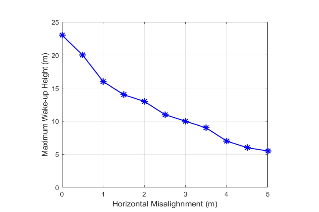
The measured wake-up height decreases as horizontal separation grows. That geometry becomes important when specifying how closely the UAV must pass a sensor.
Reading the axes. The horizontal axis is the UAV’s offset from the ground device; the vertical axis is the maximum height at which wake-up still succeeds. Each point represents a tested geometry, rather than a trajectory through time.
What the trend means. The available wake-up height drops as the UAV moves sideways. Greater separation and a less favorable line-of-sight geometry reduce the received signal, so directly overhead range cannot be assumed at every horizontal offset.
 Expand figure ↗
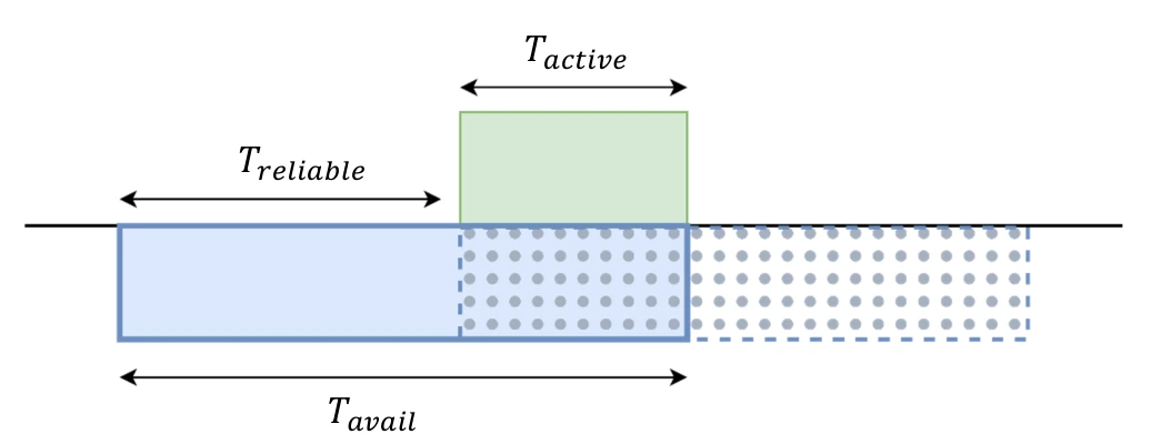
A UAV is only within range for a limited interval, and a duty-cycled sensor is active for only part of that time. The timing diagram explains why overlap determines successful communication.
Three time intervals. The device’s active interval must fit within the UAV’s available communication time. The reliable arrival window identifies timings that leave enough overlap to complete the exchange.
 Expand figure ↗
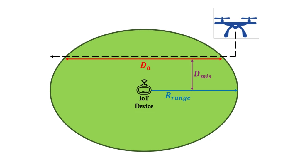
The path diagram relates UAV travel distance, radio range, and horizontal misalignment. It provides the geometry needed to translate speed into an available communication time.
Flight geometry. The path crosses the device’s communication disk with a horizontal offset. Increasing that offset shortens the traversed chord and therefore the available contact time at a fixed UAV speed.
 Expand figure ↗
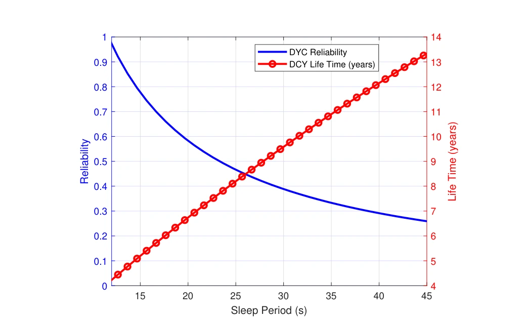
Increasing the sleep period extends battery life but reduces the chance that an ordinary duty-cycled node catches the UAV visit. The two curves make the competing effects visible.
Two vertical axes. The blue curve tracks communication reliability and the red curve battery lifetime as the duty-cycle sleep period increases. The same setting must be read against both outcomes.
The tradeoff. Longer sleep saves energy but increases the chance of missing the aircraft’s communication window. The plot therefore connects a battery-life benefit to a loss in timely availability.
 Expand figure ↗
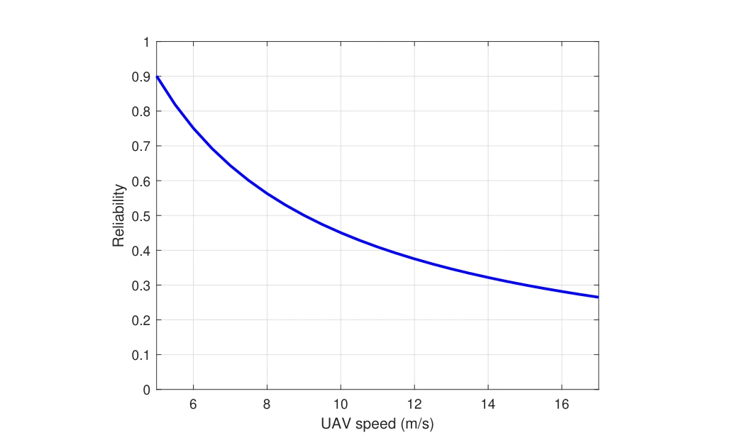
Communication reliability is plotted against UAV speed for the duty-cycled baseline. A shorter contact window makes missed visits more likely, motivating an on-demand wake-up mechanism.
What is held fixed. The plot varies UAV speed within the duty-cycled communication model. A faster aircraft spends less time within the device’s usable range, leaving fewer opportunities for a scheduled active interval to overlap.
How to read the result. The falling curve concerns successful communication during that contact window. It does not describe a change in the device’s radio sensitivity or the aircraft’s ability to transmit.
 Expand figure ↗
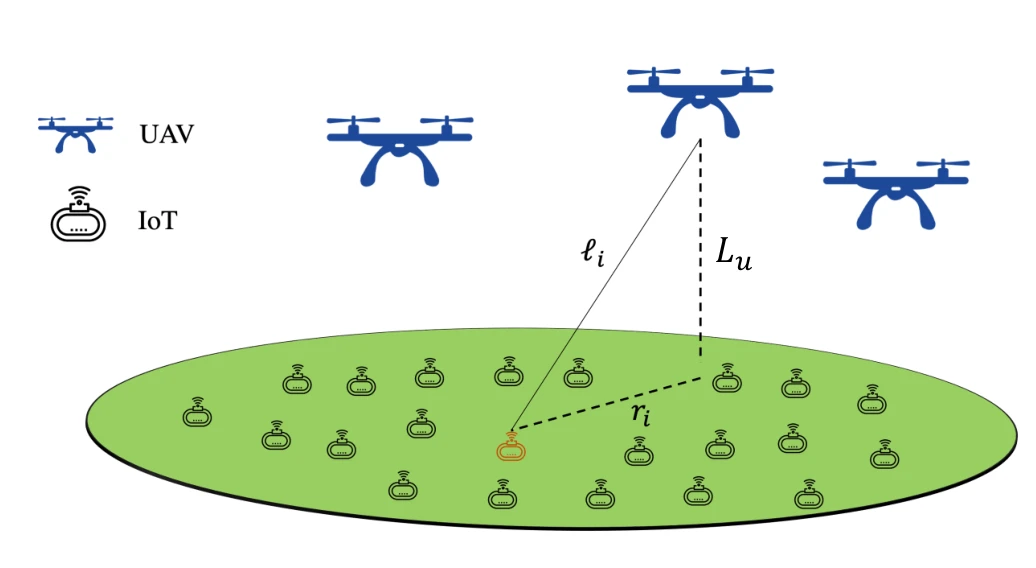
The system model expands from one UAV–sensor link to a spatial deployment. Altitude, distance, and the distribution of devices now become part of the analysis.
Spatial model. UAVs are placed above a field of IoT devices. The diagram distinguishes UAV altitude from the link distance to an individual ground node, which both enter the network geometry.
From one link to a field. The subsequent analysis averages over spatial realizations rather than assigning every device the same separation. This connects the prototype’s wake-up mechanism to probabilities of intended and unintended activation across a sensor field.
 Expand figure ↗
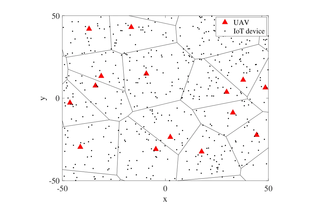
A sample field places UAVs and IoT nodes in a geometric setting. The realization illustrates the spatial assumptions used when evaluating wake-up and unintended wake-up events.
Symbols and cells. Triangles mark UAV locations and dots mark ground IoT devices. The Voronoi boundaries partition the sample field spatially, connecting an individual nearest-UAV relationship to the network model.
A spatial realization. The drawing is one realization of the assumed point processes at the stated UAV and IoT intensities. It supports the probability calculations that follow; it is not a map of a deployed agricultural site.
 Expand figure ↗
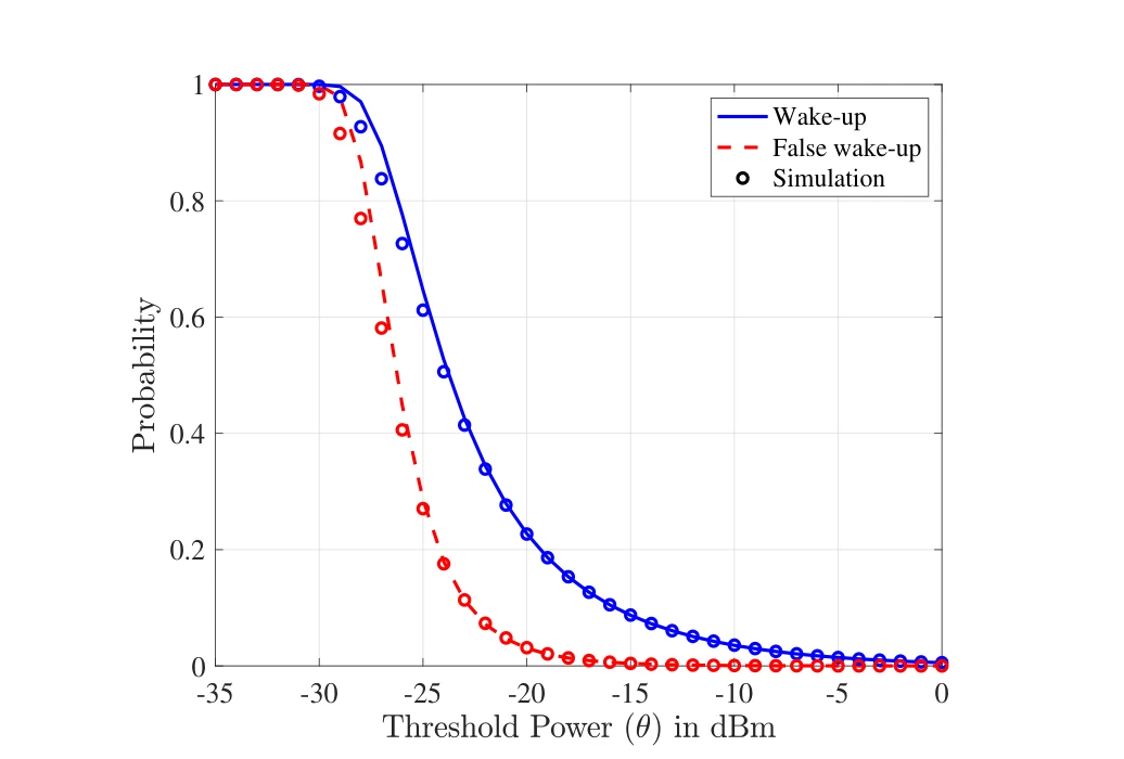
Wake-up and false wake-up probabilities respond differently to the threshold power. Simulation points provide a check on the analytical curves used to evaluate that tradeoff.
Two probabilities. The solid wake-up curve and dashed false-wake-up curve both vary with the receiver’s power threshold. Raising the threshold suppresses false activations, but also reduces the chance of detecting an intended wake-up.
Model and simulation. Simulation markers are overlaid on the analytical curves. Their comparison checks the network approximation, while the gap between the two probability curves exposes the threshold-selection tradeoff.
 Expand figure ↗
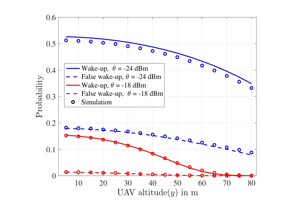
Changing UAV height alters both desired and unintended wake-up probabilities. Comparing thresholds shows why a deployment setting must consider more than communication range alone.
Across thresholds. The two threshold choices, −24 dBm and −18 dBm, give separate wake-up and false-wake-up curves. Comparing a threshold pair holds the receiver setting fixed while the UAV altitude changes.
Reading the tradeoff. Both probabilities tend to decrease with greater altitude in this model. Lower false-wake-up probability is therefore accompanied by weaker intended detection, rather than being a free improvement in selectivity.
 Expand figure ↗
The final network-scale comparison varies UAV intensity and power-conversion efficiency. It connects local receiver behavior to the probability that a device is activated across a distributed deployment.
Across UAV densities. The horizontal axis varies the UAV point-process intensity. More nearby transmitters increase the opportunity for intended wake-up, but also increase the probability of unintended activation.
Across conversion efficiencies. Separate curve pairs use power-conversion coefficients of 1 and 0.7. Comparing them connects the network-level probabilities to receiver efficiency instead of treating the radio hardware as an ideal energy converter.
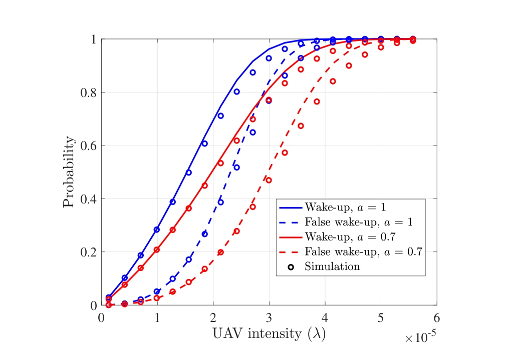 Expand figure ↗
Putting it together
The figures build from circuit and board design to measured reach, timing constraints, and network-scale probabilities. That progression connects an implemented device to the tradeoffs needed for a larger aerial sensing system.
Khalifa, O., Mohammed, A. S., Alhejab, A., Abdelrahman, A. S., Al-Radhwan, A., Zhagypar, R., ElSawy, H., Kouzayha, N., Al-Harthi, N., Elmirghani, J., Aksoy, Z., & Al-Naffouri, T. Y. Energy-Efficient Aerial Data Aggregation for IoT: From Prototyping to Large-Scale Implementation. IEEE Transactions on Instrumentation and Measurement, 74, 1-18 (2025).
@article{khalifa2025aerial,
  title = {Energy-Efficient Aerial Data Aggregation for IoT: From Prototyping to Large-Scale Implementation},
  author = {Khalifa, Omar and Mohammed, Anas S. and Alhejab, Ali and Abdelrahman, Abdelrahman S. and Al-Radhwan, Ahmed and Zhagypar, Ruslan and ElSawy, Hesham and Kouzayha, Nour and Al-Harthi, Noha and Elmirghani, Jaafar and Aksoy, Zekeriya and Al-Naffouri, Tareq Y.},
  journal = {IEEE Transactions on Instrumentation and Measurement},
  volume = {74},
  pages = {1--18},
  year = {2025},
  doi = {10.1109/TIM.2024.3497061}
}
Anas S. Mohammed1, Omar Khalifa2, Ali Alhejab2, Abdelrahman S. Abdelrahman1, Ahmed Al-Radhwan1, Hesham ElSawy3, Nour Kouzayha2, Noha Al-Harthi4, Jaafar Elmirghani4, Mansoor Hanif4, Tareq Y. Al-Naffouri2
An IoT node need not stay fully awake while waiting for a data-collection visit. This demonstration combines an addressed wake-up receiver, a UAV-carried transmitter, and a dashboard. Its figures document the system, outdoor range testing, the sensing board, and the end-to-end demonstration.
The system diagram follows the wake-up signal from the UAV to an IoT device, then follows the collected data to the base station and user interface. It also shows the hardware path used to detect an addressed wake-up call.
System path. The UAV activates a ground device through the wake-up link, then relays its measurements toward the base station and dashboard. The arrows distinguish activation from sensed-data transfer.
Receiver detail. The inset places signal conditioning and address detection before the main sensing and communication circuitry. This separation explains how the device can wait for a call without keeping its full data path active.
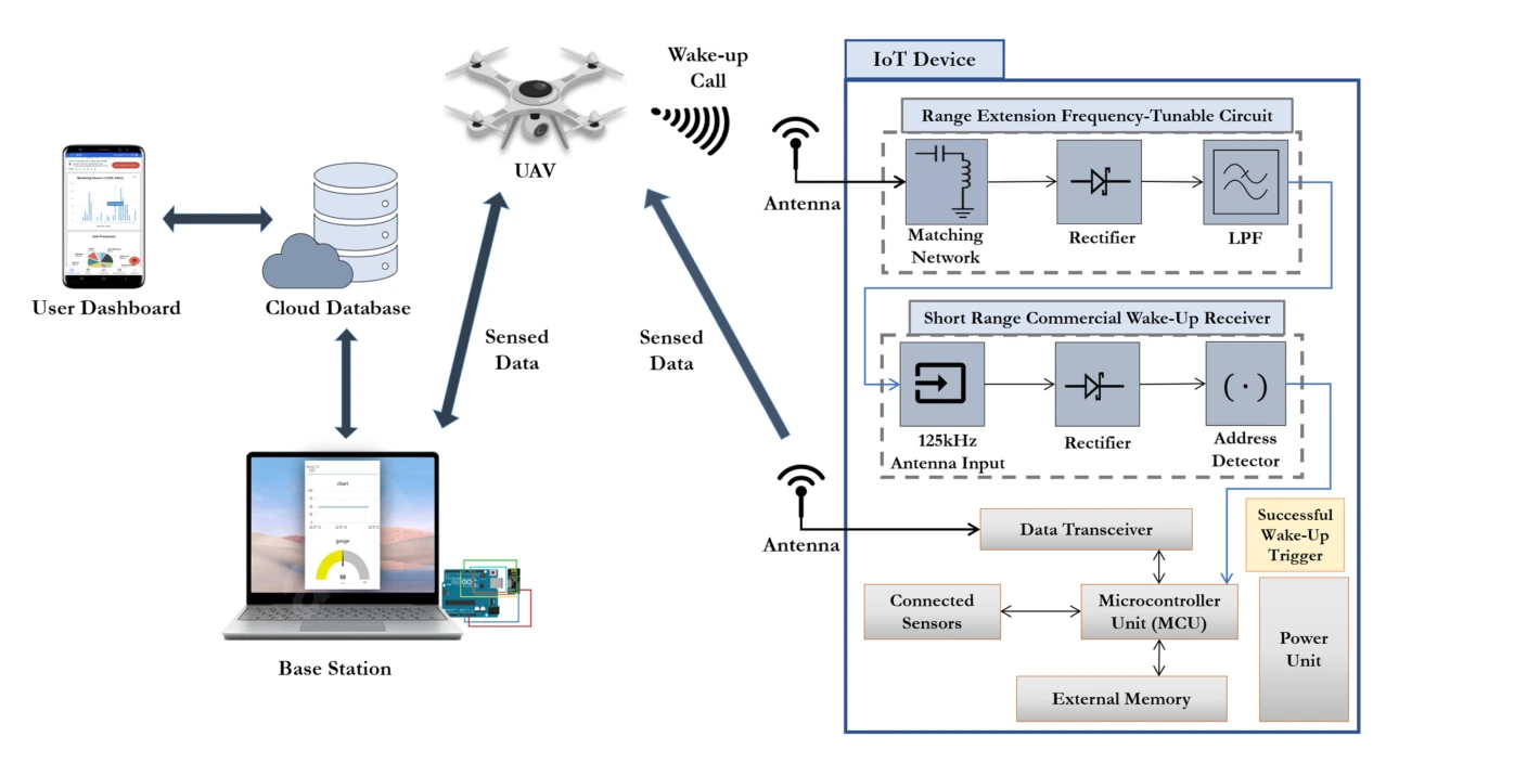 Expand figure ↗
The field setup places the transmitter on a UAV and the receiving node on the ground. This makes aerial reach and alignment part of the practical system test.
Outdoor arrangement. The transmitter is carried by the UAV while the receiver is part of the ground IoT node. This places the wake-up mechanism in the geometry relevant to aerial data collection, beyond an instrument-only bench test.
What is evaluated. The experiment tests successful device wake-up as the aircraft’s position changes. The later height-versus-offset plot is needed to interpret the operating range; the setup photograph establishes where the transmitting and receiving hardware are located.
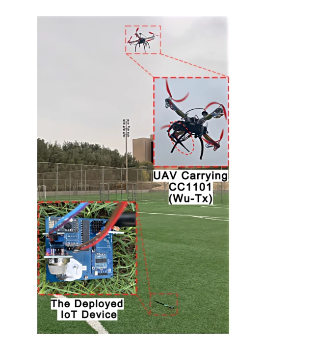 Expand figure ↗
The board brings together sensors, a microcontroller, a data transceiver, and the wake-up receiver. These components allow a sleeping node to respond to a call and then transmit its measurements.
Board functions. The labeled blocks locate the microcontroller, wake-up receiver, data transceiver, battery, and sensor connections. They show the complete sensing node used in the demonstration.
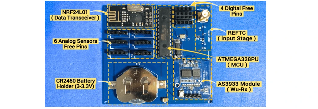 Expand figure ↗
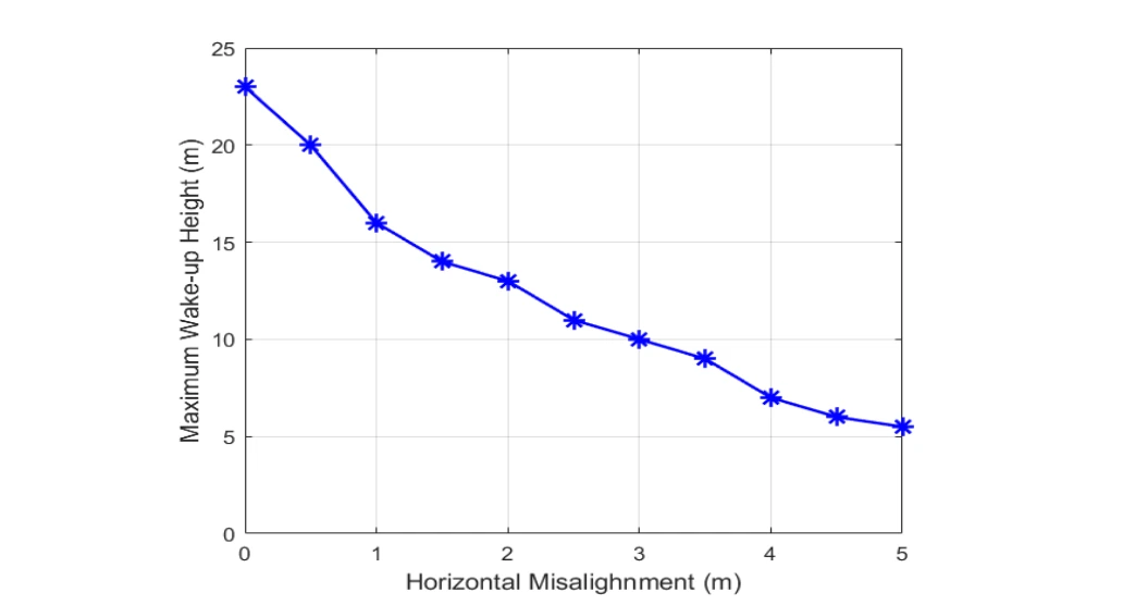
The maximum wake-up height is plotted as the UAV moves away from direct alignment with the device. The result turns a laboratory communication link into a deployment constraint.
Geometry and range. The vertical axis is the maximum successful wake-up height; the horizontal axis is sideways offset from the device. Each point describes a different link geometry, rather than flight time.
Observed trend. The tested height falls as offset increases. This distinguishes the favorable overhead case from operation farther to one side, where greater separation and antenna alignment constrain the link.
 Expand figure ↗
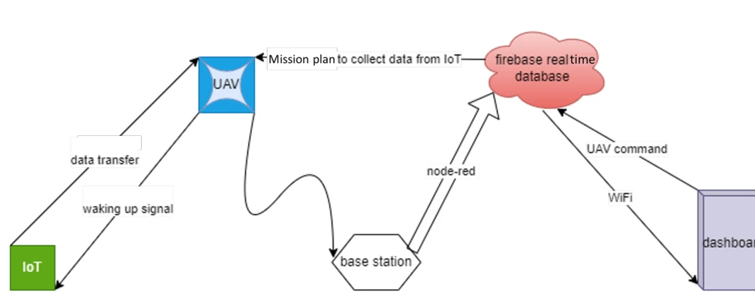
The data-flow diagram connects flight control, sensing, the base station, a cloud database, and the dashboard. It shows how the radio event becomes information visible to a user.
Measurements and commands. Measurements move through the UAV/base-station link to a Firebase database and dashboard. The command path lets the interface request an intended node, with Node-RED linking the software components.
 Expand figure ↗
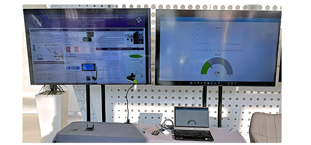
The workstation setup places monitoring and control interfaces alongside the physical electronics. This is the integration step that connects individual working components into a usable system.
Demonstration setup. The raised transmitter emulates the UAV side during an indoor demonstration. The laptop and displays show the collected data and interface, allowing the wake-up/data sequence to be inspected without flying an aircraft in the venue.
 Expand figure ↗
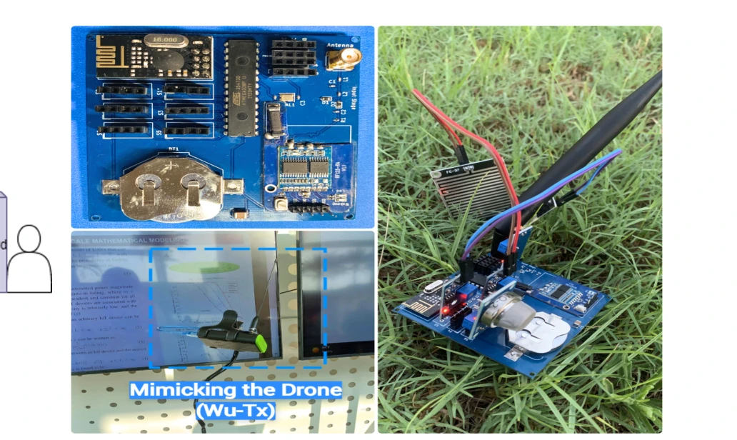
The final photographs show the IoT node and a controlled UAV-emulation setup. They document the practical activation and data-collection process used in the demo.
The sensing device. The 7 × 7 cm² IoT board combines the low-power wake-up path with the circuitry needed to acquire and transmit measurements. The board is the end device being activated, rather than a stand-in for the radio link.
The demonstration. The setup emulates the UAV-side wake-up transaction so visitors can follow activation and data collection. This makes the sequence inspectable in a demonstration setting, alongside the separate outdoor range experiments.
 Expand figure ↗
Putting it together
The demonstration establishes a complete wake-up-and-collect workflow. The later journal study expands this foundation with device engineering, reliability analysis, and large-scale network modeling.
Mohammed, A. S., Khalifa, O., Alhejab, A., Abdelrahman, A. S., Al-Radhwan, A., ElSawy, H., Kouzayha, N., Al-Harthi, N., Elmirghani, J., Hanif, M., & Al-Naffouri, T. Y. Demo Abstract: Energy-Efficient Aerial Data Aggregation in IoT Networks with WuR. IEEE International Black Sea Conference on Communications and Networking, 147-149 (2023).
@inproceedings{mohammed2023wur,
  title = {Demo Abstract: Energy-Efficient Aerial Data Aggregation in IoT Networks with WuR},
  author = {Mohammed, Anas S. and Khalifa, Omar and Alhejab, Ali and Abdelrahman, Abdelrahman S. and Al-Radhwan, Ahmed and ElSawy, Hesham and Kouzayha, Nour and Al-Harthi, Noha and Elmirghani, Jaafar and Hanif, Mansoor and Al-Naffouri, Tareq Y.},
  booktitle = {2023 IEEE International Black Sea Conference on Communications and Networking (BlackSeaCom)},
  pages = {147--149},
  year = {2023},
  doi = {10.1109/BlackSeaCom58138.2023.10299765}
}
Tarig Ballal1, Abdelrahman S. Abdelrahman2, Ali H. Muqaibel2, Tareq Y. Al-Naffouri1
The minimum-variance portfolio depends on an inverse covariance matrix, which can amplify estimation noise. This paper reformulates the weights and adapts the regularization parameter to the observed returns. Two data experiments examine the resulting realized risk across training-window lengths and added noise levels.
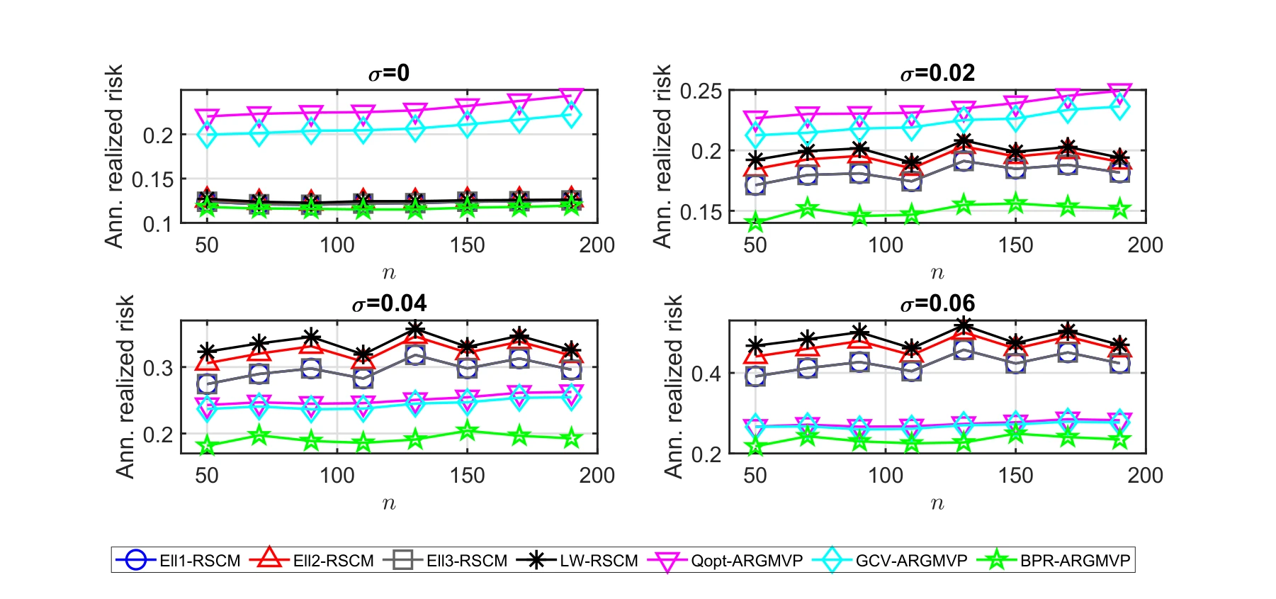
The first experiment uses 45 Hang Seng Index assets observed from 2010 to 2011. Each panel varies the added noise level, comparing annualized realized risk across training-window lengths and competing covariance-regularization methods.
The four plots. The panels add Gaussian return noise with standard deviations 0, 0.02, 0.04, and 0.06. Each plots annualized realized risk against the training-window length for the 2010–2011 asset set.
What to compare. Lower risk is the evaluation criterion. Comparing methods at the same window length and noise setting tests sensitivity to noisy returns, rather than comparing different training histories.
 Expand figure ↗
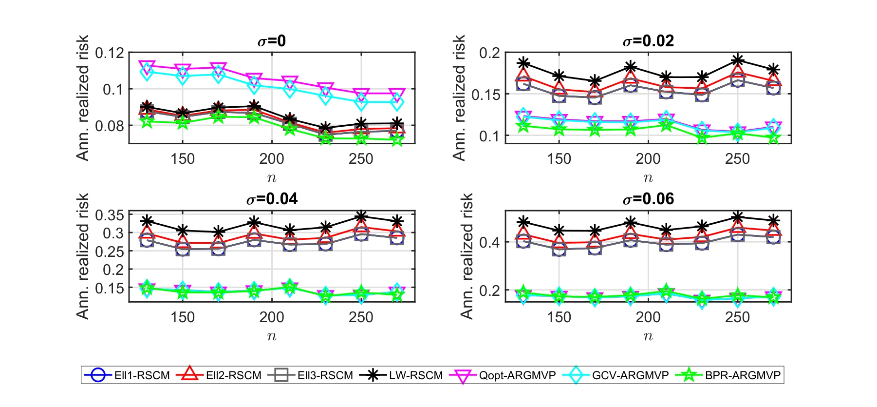
A second experiment uses 50 Hang Seng Index assets from 2016 to 2017. Repeating the noise and training-window comparisons checks whether the behavior carries over to a different asset set and time period.
A second dataset. The same four noise settings are evaluated on the 2016–2017 period with 50 assets. The repeated design checks whether the pattern from the earlier period persists on another dataset.
Reading the curves. Compare methods within each panel before comparing noise levels. These are realized-risk results for the tested historical datasets, rather than a guarantee about future portfolio performance.
 Expand figure ↗
Putting it together
The figures evaluate the proposal through out-of-sample realized risk rather than matrix estimation alone. The central idea is to make the regularization parameter respond to the data used to construct the portfolio.
Ballal, T., Abdelrahman, A. S., Muqaibel, A. H., & Al-Naffouri, T. Y. An Adaptive Regularization Approach to Portfolio Optimization. ICASSP - IEEE International Conference on Acoustics, Speech and Signal Processing, 5175-5179 (2021).
@inproceedings{ballal2021adaptive,
  title = {An Adaptive Regularization Approach to Portfolio Optimization},
  author = {Ballal, Tarig and Abdelrahman, Abdelrahman S. and Muqaibel, Ali H. and Al-Naffouri, Tareq Y.},
  booktitle = {ICASSP 2021 — 2021 IEEE International Conference on Acoustics, Speech and Signal Processing (ICASSP)},
  pages = {5175--5179},
  year = {2021},
  doi = {10.1109/ICASSP39728.2021.9413865}
}
02 / Teaching & mentorship
From executable sampling notebooks to digital circuits and student research. Courses, materials, and mentorship at UC Santa Barbara.
Mentored a four-week protein-folding project, from an HP lattice environment and REINFORCE benchmarks to a final report and presentation.
Mentored a student on Protein Folding Using Variational Annealing over four weeks. Guided problem formulation, a tested HP lattice-folding environment, REINFORCE baselines and benchmarks, and the final report and presentation.
Accelerated Convergence in Glassy Energy Landscapes via Variational Learning
The proposal explores gradient-estimating and learning-based optimization for protein folding and spin-glass models. Instead of adjusting a candidate solution alone, it treats combinatorial optimization as learning a probability distribution over discrete configurations.
Two questions guide the proposed work:
The proposed outcomes are an optimization algorithm, an implementation benchmarked against derivative-free methods, and a technical report documenting the methodology and results.
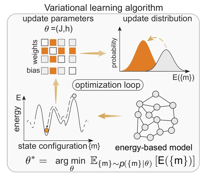
Designed and taught INT 93LS–001, with lecture notes and executable notebooks on sampling, discrete optimization, and stochastic neural networks.
Designed and taught INT 93LS–001: Probabilistic Computing, an intensive UCSB summer course. Students explored Monte Carlo methods, Ising and Potts models, simulated annealing, and stochastic neural networks through lecture notes and executable notebooks.
Advancing Scalable and Energy-Efficient Machine Intelligence
Summer Research Academies · Track 1 · INT 93LS–001
The course examines how randomness can become a useful computing resource as conventional systems encounter limits in power use and physical scaling. Students connect probability, linear algebra, optimization, and machine learning to algorithms designed for efficient computation.
Through Python implementations, students study Markov chain sampling with Gibbs and Metropolis–Hastings methods, then use simulated annealing and parallel tempering to tackle combinatorial optimization. The emphasis is on understanding how stochastic algorithms work and evaluating the computational benefits they can offer.
The course also applies probabilistic methods to neural networks. Students train stochastic models, compare them with deterministic baselines, and examine the trade-offs among accuracy, runtime, and energy use. They leave with practical experience building probabilistic algorithms and assessing when engineered randomness is useful for machine intelligence.
Source: UCSB Summer Sessions track listing, saved November 3, 2026.
Timing diagrams, propagation delay, latches and flip-flops, shift registers and counters, finite state machines, Verilog, two-phase clocking, and timing analysis.
Led discussion sections and labs covering timing diagrams, propagation delay, latches and flip-flops, shift registers and counters, Mealy/Moore finite state machines, Verilog, two-phase clocking, and timing analysis.
A recorded ECE 152A demonstration of the seven-segment display circuit in Logisim, from the lab materials. Open demo ↗
Continuous-time linear systems in time and frequency domains, including convolution, Laplace transforms, and Fourier transforms.
Led discussion and lab support for continuous-time linear systems in time and frequency domains, including convolution, Laplace transforms, and Fourier transforms.
Matrix arithmetic, vector spaces, orthogonality, factorizations, determinants, eigenvalues and eigenvectors, and difference and differential equations.
Led student support for applied linear algebra topics including matrix arithmetic, vector spaces, orthogonality, matrix factorizations, determinants, eigenvalues and eigenvectors, and difference and differential equations.
03 / Applied work
Computer vision systems developed at Wakeb for industrial safety and real-time monitoring.
Alfanar Electric / Smart Alerting System
Personnel detection in high-voltage test areas, enabling automated safety shutdowns.
Saudi Water Authority / Aware
A PyTorch and YOLO crowd-management system with a secure offline dashboard for autonomous operation.
04 / Background
Education, experience, technical skills, awards, and the talks that connect the ideas.
Download full CV ↗Handshake AI Fellow — Trainer and Reviewer
Completed 20+ graduate-level STEM benchmark problems, each rated 5/5 across three review stages. Developed long-form AI evaluations for electrical and computer engineering workflows.
Graduate Student Researcher, OPUS Lab, UCSB
Research and paper stories ↗Data Scientist, Computer Vision, Wakeb
Deployed computer vision systems ↗Researcher, Neurotronics Lab, KFUPM
Lab profile ↗Research Intern, Information Science Lab, KAUST
KAUST profile ↗