The question
Two coupled oscillators can exchange energy in ways that resemble a two-level system. Adding a delay changes the mode spectrum and stability of that exchange. The paper follows the connection from a mechanical model through eigenvalue structure to time-domain energy dynamics.
Define the delayed oscillator pair.
A two-mass spring model establishes the degrees of freedom, damping, and coupling. It provides a classical setting in which the consequences of finite interaction delay can be studied explicitly.
Model components. The masses and wall springs define the uncoupled oscillators; the coupling and damping terms determine how their motion interacts and decays.

See the spectral modes without delay.
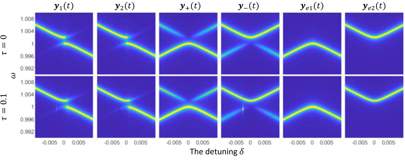
Power spectra for several history functions establish the reference response. Detuning changes which modes are excited and how their resonances appear in the total spectral density.
Upper and lower panels. The upper spectra use zero delay; the lower spectra use a delay of 0.1. Different history functions excite different mode combinations, so comparing rows separates delay effects from the initial preparation.
Connect the spectrum to energy trajectories.
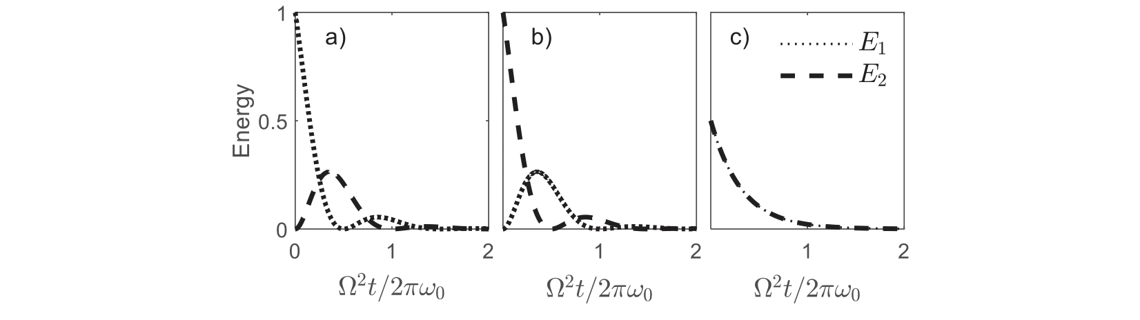
The oscillator energies are plotted for different initial histories. These time-domain examples show how the chosen preparation changes the visible exchange between the two subsystems.
Panels (a)–(c). Three history functions prepare the same coupled system differently. Following both energy curves shows how the preparation changes the observed exchange without changing the model parameters.
Track damping through spectral linewidths.
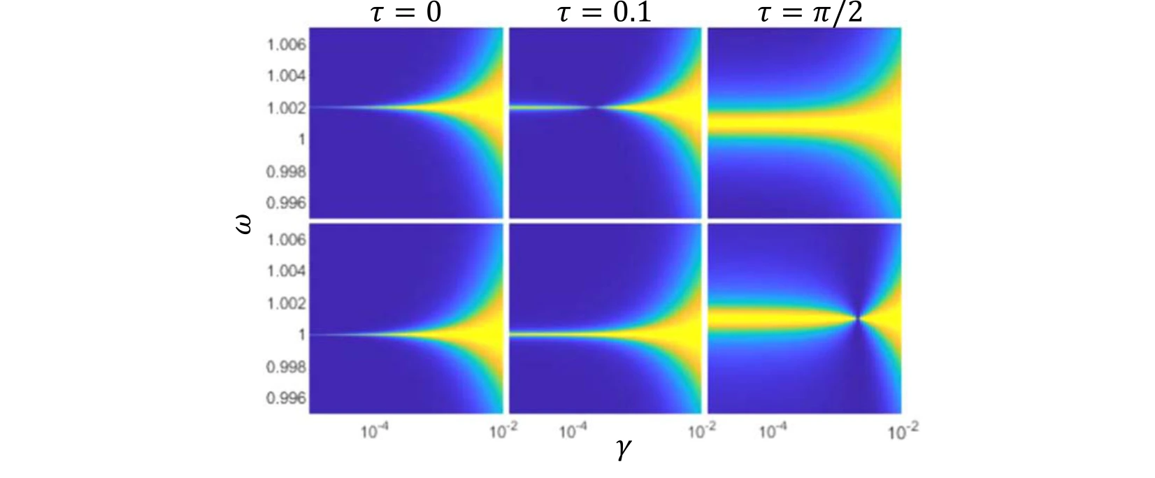
Linewidths of the coupled modes are compared across damping rates and delays. This connects the spectral response to the persistence of the oscillations.
Upper and lower panels. The upper plots follow the second eigenstate and the lower plots the first. Comparing delays at the same damping rate reveals changes in spectral linewidth.
Follow the delayed eigenvalue spectrum.
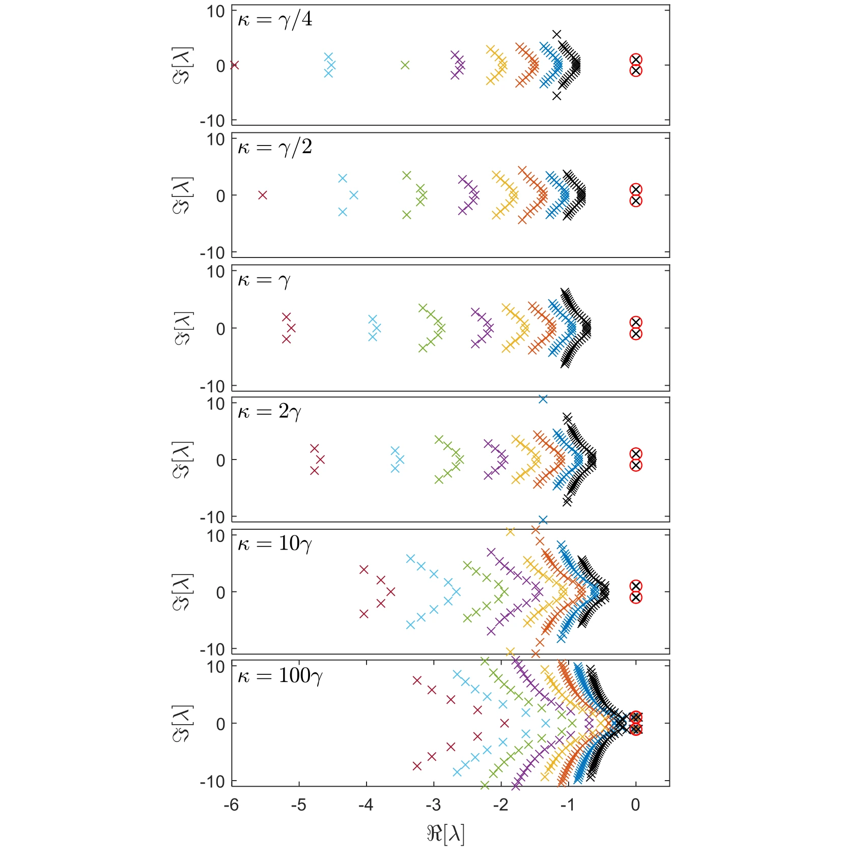
The complex spectrum is plotted for different couplings and delays. Moving beyond the instantaneous model reveals additional structure in the possible dynamical modes.
Across the six rows. The coupling increases from one quarter of the damping rate to one hundred times that rate. Within each row, colors distinguish delays from 0.3 to 1.0, allowing the displacement of the spectrum to be separated from a change in coupling.
The red circles. The two highlighted roots are the main dynamical modes followed in the later figures. Their horizontal position gives the growth or decay rate, while their vertical position gives the oscillation frequency.
Reading the comparison. Use the same axes to compare the circled pair with the other roots. The figure establishes which part of the spectrum is being tracked before subsequent plots focus on the dominant pair and the stability boundary.
Resolve the principal eigenvalues as delay changes.
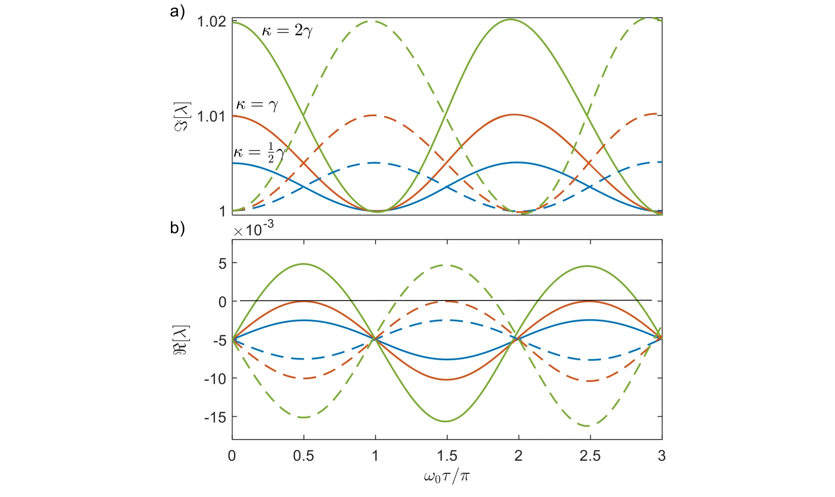
Real and imaginary parts of the main modes are followed across delay. Their trajectories distinguish changes in oscillation frequency from changes in stability or decay.
Real and imaginary components. The two plots separate changes in decay or growth from changes in oscillation frequency. Solid and dashed curves of the same color identify the two main modes at a fixed coupling.
The stability boundary. The black zero-real-part line marks the transition between decay and growth. Comparing the three coupling choices—half, equal to, and twice the damping rate—shows why frequency splitting alone does not establish stable dynamics.
Identify the modes that control long-time behavior.
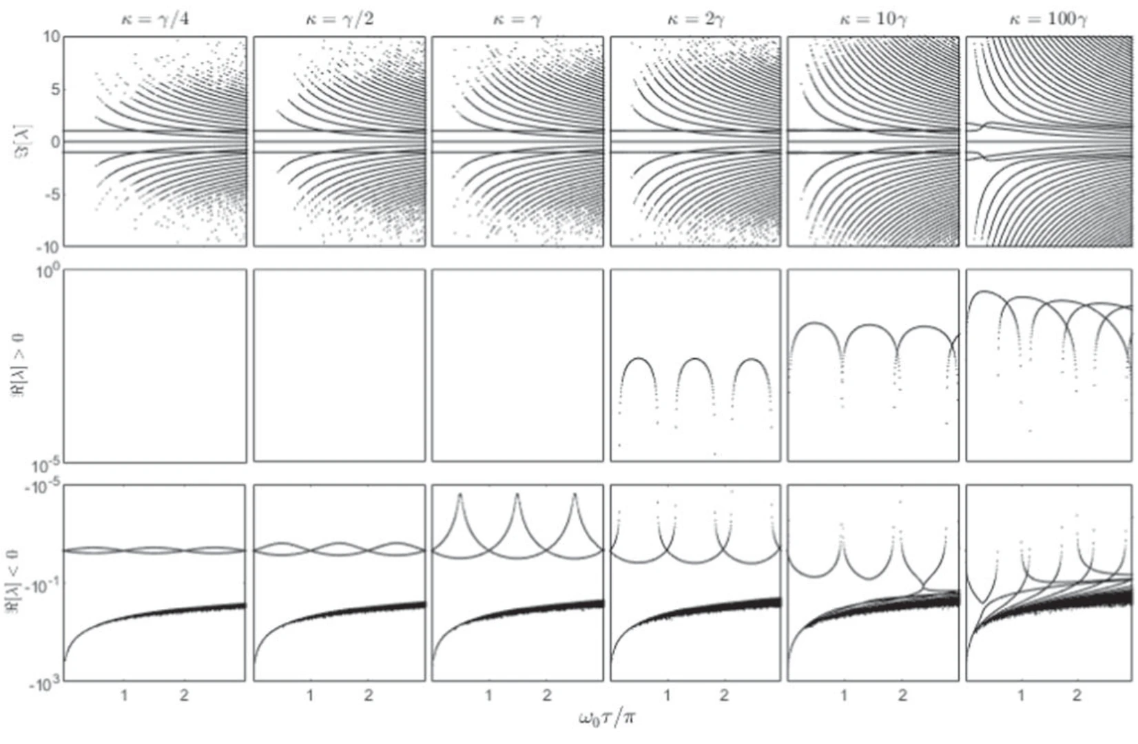
The rightmost eigenvalues determine whether a mode grows or decays most slowly. Comparing coupling strengths exposes how the dominant dynamical behavior changes with delay.
Top row. The imaginary parts track oscillation frequencies as normalized delay changes. Following both branches reveals how the dominant pair evolves across the tested coupling strengths.
Middle and bottom rows. Positive real parts are plotted separately from negative real parts. That separation makes unstable growth distinguishable from damped motion, even when their frequency branches look similar.
View mode evolution in the complex plane.
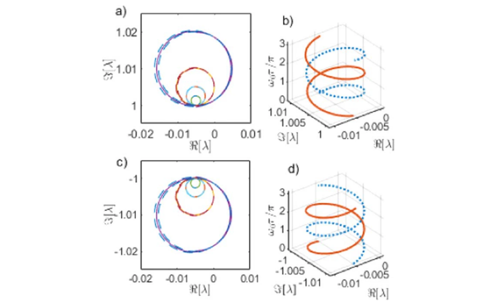
The eigenvalue paths offer another representation of the same delayed dynamics. Their geometry clarifies how conjugate modes move as the interaction delay varies.
Panels (a) and (b). These trajectories follow the upper pair of coupled modes in the complex plane. Read horizontal displacement as a change in the real part and vertical displacement as a change in frequency.
Panels (c) and (d). The lower panels show the corresponding conjugate modes. Viewing the pairs together links the separate real- and imaginary-part plots to complete eigenvalue trajectories as delay varies.
Summarize the geometry of the mode paths.
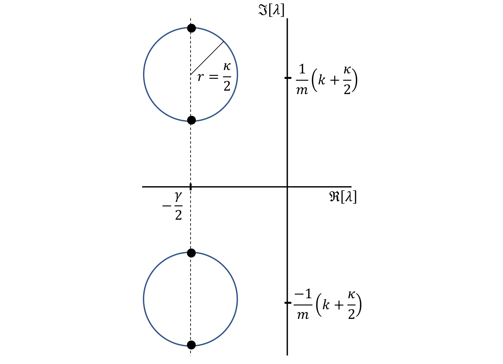
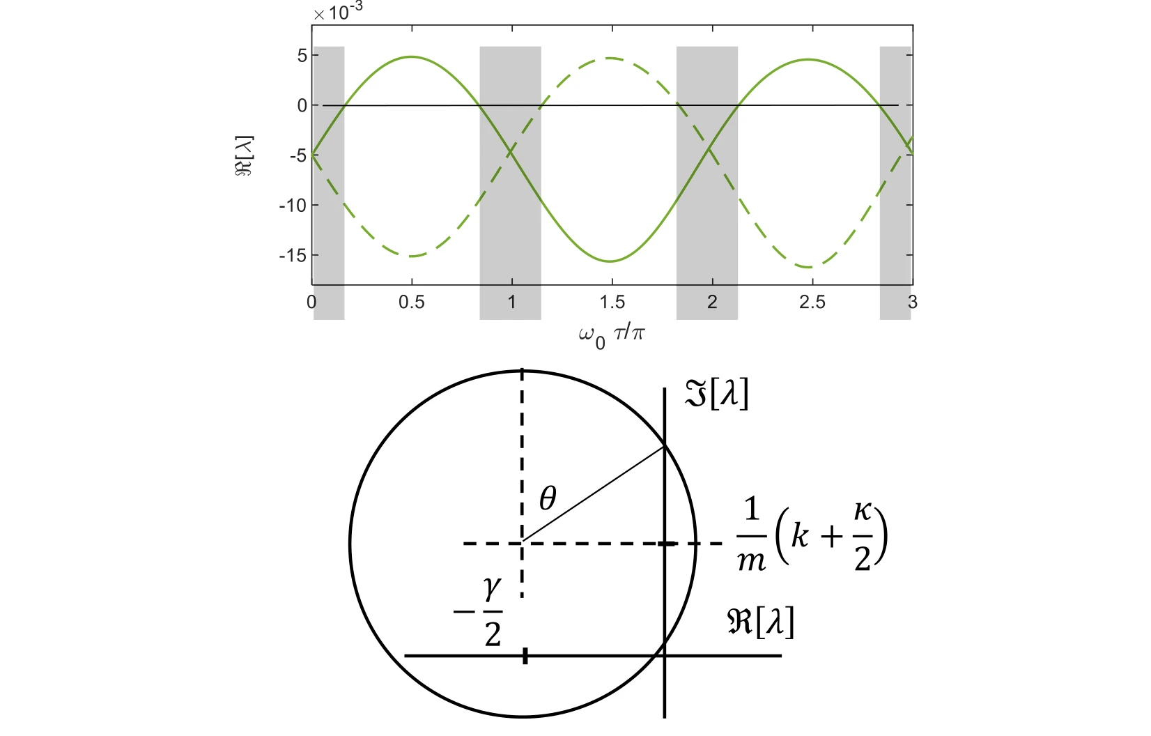
A schematic condenses the evolution into circles and interwinding trajectories. It provides a visual guide to the more detailed eigenvalue plots that precede it.
Reading the schematic. The circles summarize the mode paths in the preceding complex-plane plots. Their overlap and interwinding organize the recurring evolution with delay; the drawing is a geometric guide to those trajectories, rather than another time-domain measurement.
Locate intervals of instability.
The stability map gathers intervals in which eigenvalues imply growing motion. Comparing different coupling strengths shows how stable and unstable delay ranges alternate.
Stable intervals. Gray intervals in the upper panel mark stable dynamics. Comparing their widths and locations as coupling increases makes the repeated stable and unstable delay regions easier to identify than in individual root plots.
Connection to the spectrum. These intervals summarize where the leading eigenvalues have the sign required for decay. They should be read together with the real-part plots, which show how a mode reaches the stability boundary.
Connect stability boundaries to bifurcation.
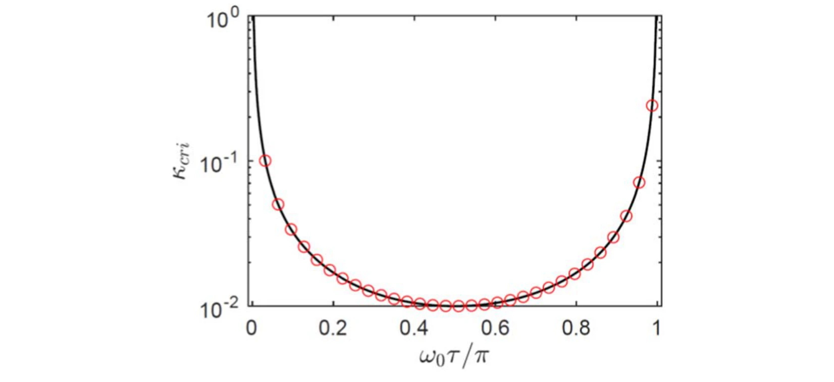
A bifurcation diagram plots the critical coupling against normalized delay. It connects the observed stability transitions with the boundary predicted by the dynamical analysis.
Curve and markers. The black bifurcation boundary plots critical coupling against normalized delay. Red circles evaluate the derived stability condition, providing a direct check against that boundary.
Revisit the spectrum in the delayed regime.
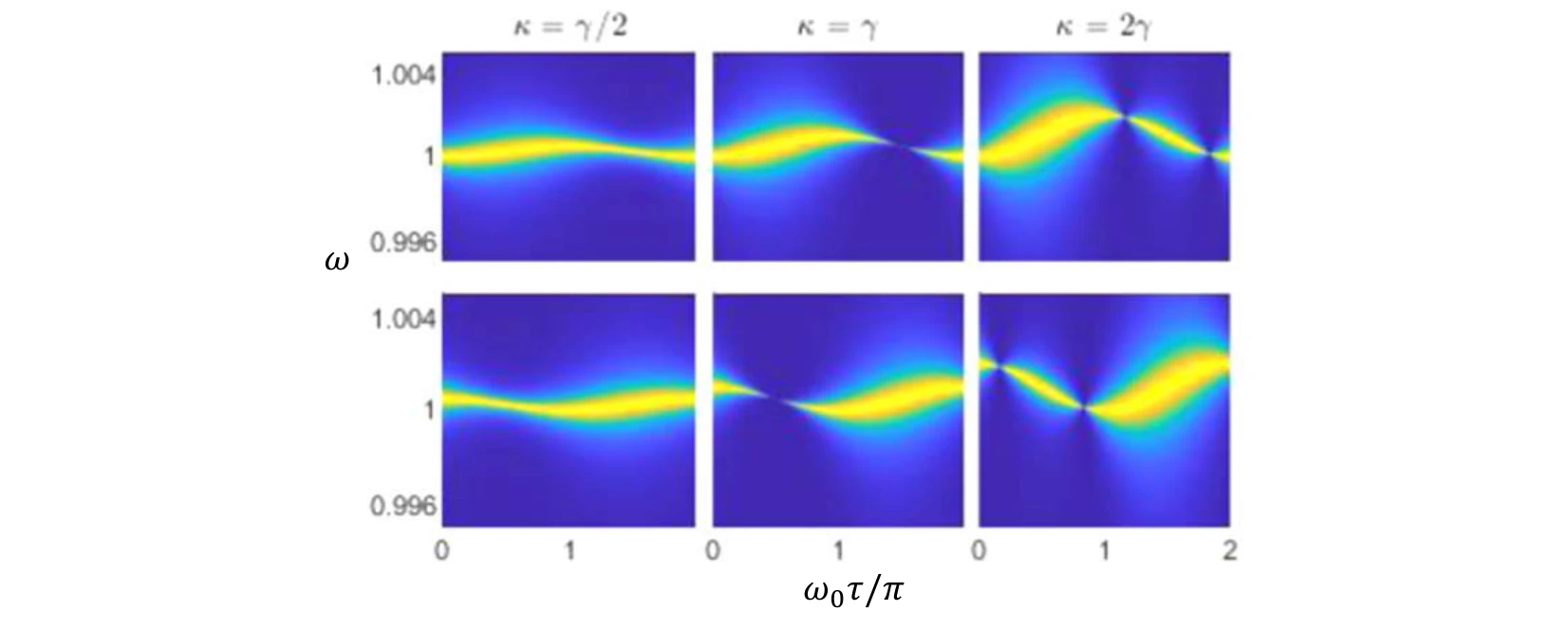
Power-density plots compare several coupling cases and history functions as delay varies. They connect changes in the eigenvalue picture to observable spectral features.
Rows and columns. The rows correspond to the two eigenstates. The three coupling choices—half, equal to, and twice the damping rate—show how the delay-dependent spectra change across the coupling boundary.
Measure energy exchange and coherence.
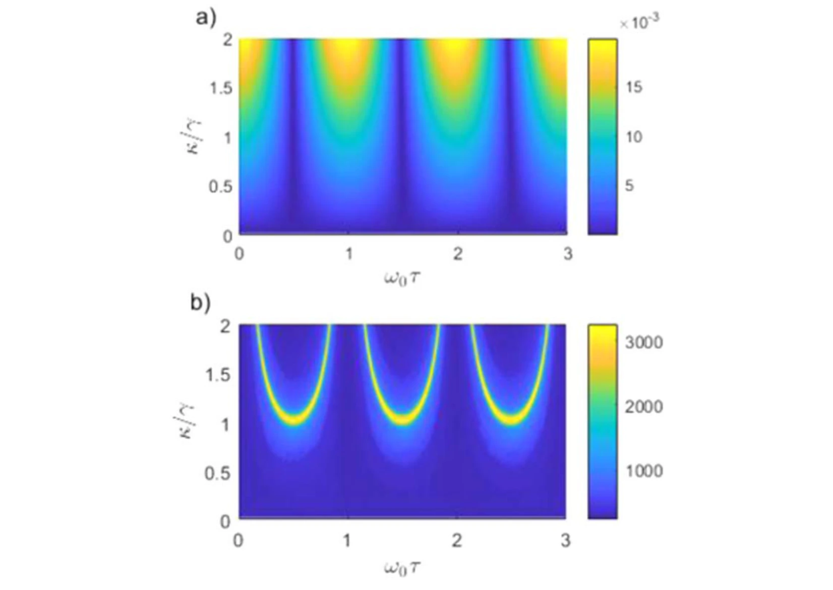
The exchange frequency and coherence time are mapped across coupling and delay. These quantities summarize how quickly energy moves and how long the exchange remains discernible.
Panel (a). The energy-exchange frequency is plotted against both coupling and delay. It describes how quickly energy moves between the oscillators; it is a different quantity from the individual oscillators’ carrier frequencies.
Panel (b). The coherence-time surface measures how long the exchange remains coherent under the same parameter variation. Comparing the surfaces separates a faster transfer process from a longer-lived one.
Inspect trajectories near the coupling boundary.
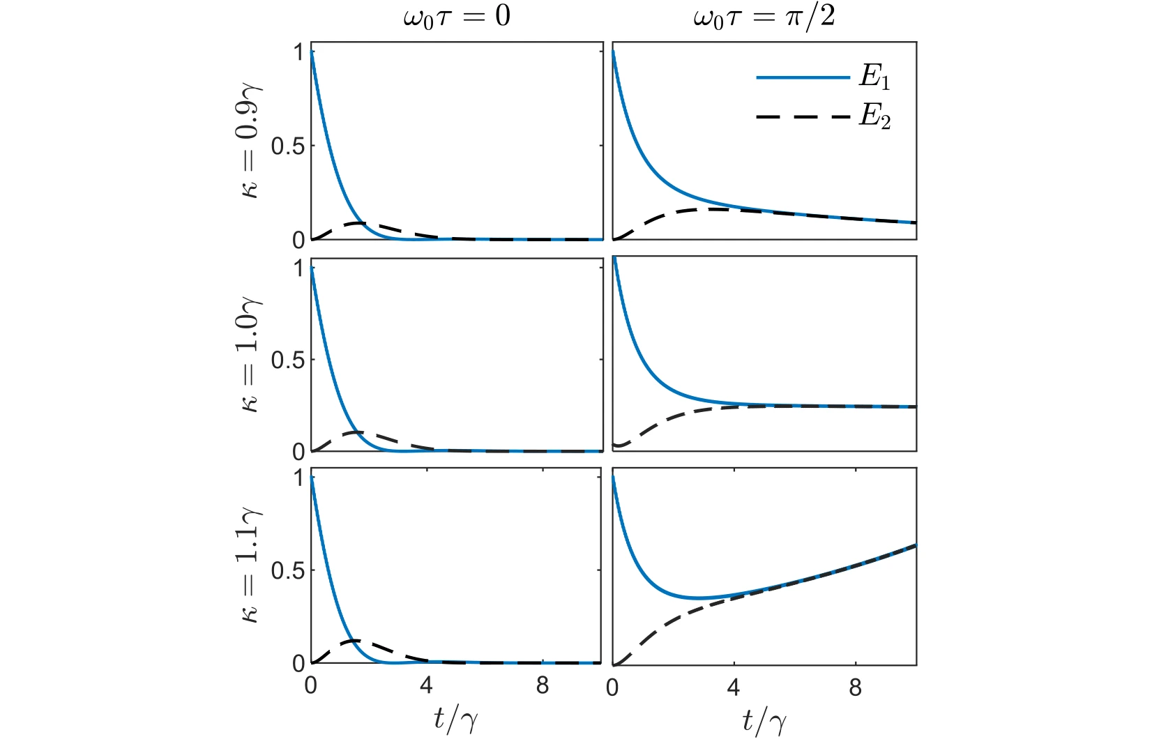
Time traces compare the individual oscillator energies for couplings around the damping scale. The cases place the abstract coherence and stability measures back into direct energy dynamics.
Across the rows. The coupling is 0.9, 1.0, and 1.1 times the damping rate. These closely spaced choices probe the region around the coupling boundary instead of comparing only widely separated regimes.
Across the columns. The left and right columns use normalized delays of zero and π/2. Each plot follows both oscillator energies, making the effect of delay visible at the same coupling.
Compare weak and stronger coupling in time.
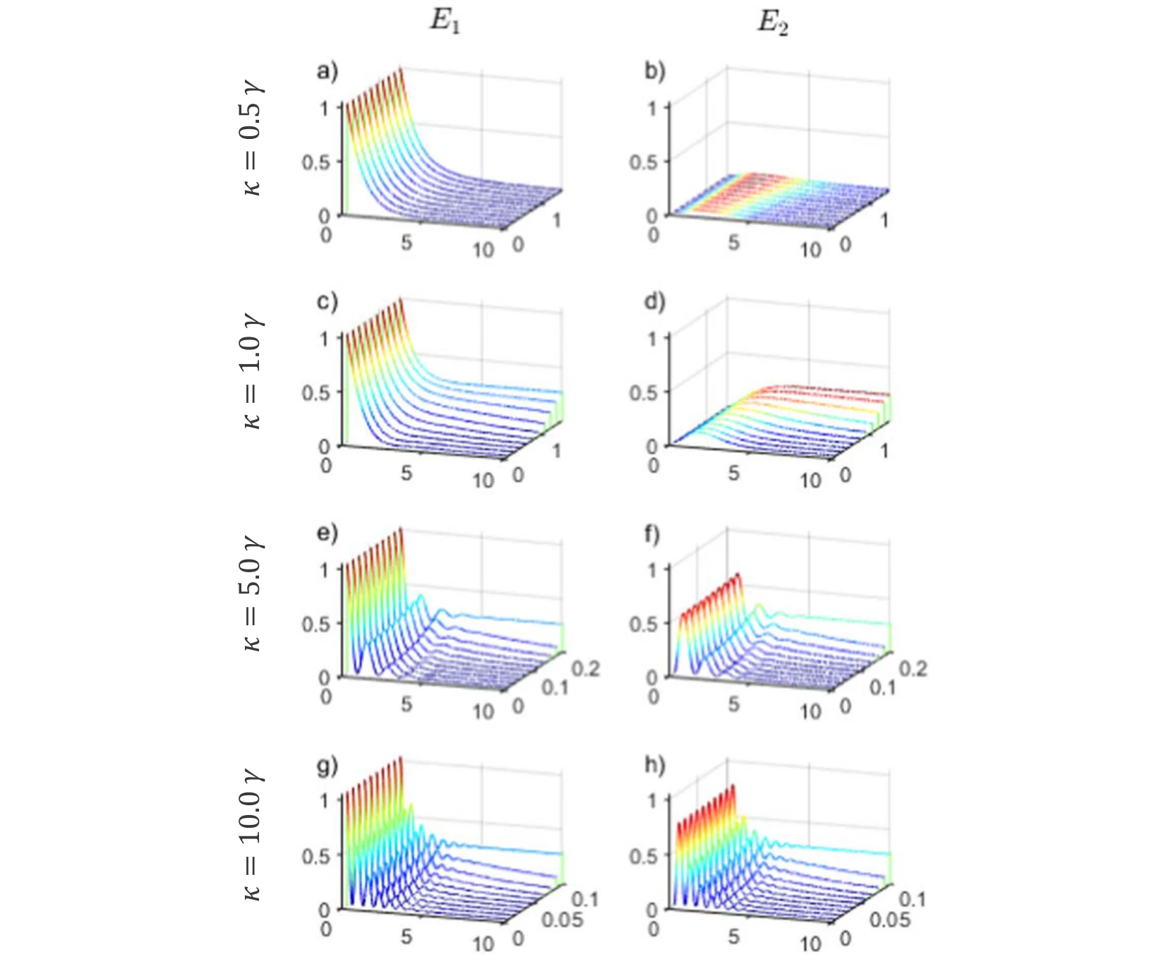
The final trajectories broaden the coupling comparison and contrast instantaneous with delayed interaction. They complete the connection between the spectrum, stability, and the observed energy exchange.
Panels (a), (c), (e), and (g). The left column shows the first oscillator’s energy. From top to bottom, coupling rises from 0.5 to 1, 5, and 10 times the damping rate, while each surface varies time and delay.
Panels (b), (d), (f), and (h). The right column follows the second oscillator under the matching conditions. Compare each row as a pair to see transferred energy alongside the energy remaining in the first oscillator.
Reading the surfaces. The oscillatory exchange becomes more apparent in the stronger-coupling rows. The plotted delay range also changes between rows, so matching the axes matters when comparing the extent and persistence of the oscillations.
Putting it together
One model, several views of the dynamics.
Spectra, eigenvalues, stability maps, and energy trajectories describe complementary aspects of the same system. Delay links these views by changing both the allowed modes and the coherence of their energy exchange.
Citation
Alharbi, F. H., Abdelrahman, A. S., Alkathiry, A. M., & Al-Qahtani, H. M. Energy Transfer and Coherence in Coupled Oscillators with Delayed Coupling: A Classical Picture of Two-Level Systems. Physica Scripta, 97(8) (2022).
BibTeX
@article{alharbi2022energy,
  title = {Energy transfer and coherence in coupled oscillators with delayed coupling: a classical picture of two-level systems},
  author = {Alharbi, Fahhad H. and Abdelrahman, Abdelrahman S. and Alkathiry, Abdullah M. and Al-Qahtani, Hussain M.},
  journal = {Physica Scripta},
  volume = {97},
  number = {8},
  pages = {085215},
  year = {2022},
  doi = {10.1088/1402-4896/ac7f62}
}