The question
Delayed interactions turn a familiar oscillator problem into a transcendental eigenvalue problem. This study compares four approximation strategies against a shared physical model, separating their predictions for the real and imaginary parts of the fundamental eigenfrequencies.
Define one physical problem for every method.
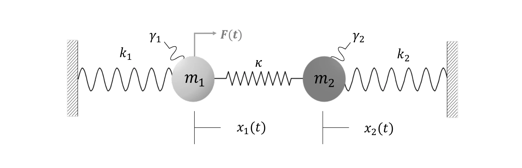
Two coupled mass–spring oscillators provide the common test system. A delay in the interaction changes the characteristic equation, making the calculation of dynamical eigenvalues more demanding than in the instantaneous case.
The common benchmark. The wall springs, masses, and coupling define one mechanical system for every solver. An external force acts on the first mass to initiate the response.
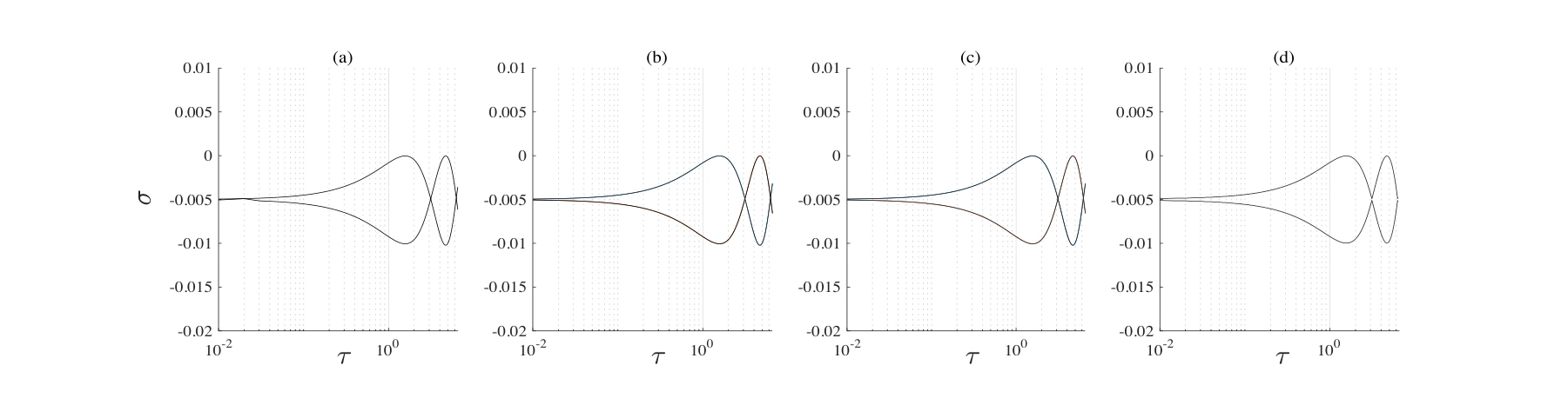
Compare the real components of the eigenvalues.
Taylor expansion, Rekasius substitution, self-consistent iteration, and Chebyshev discretization are evaluated as the delay varies. The real components reveal the predicted growth or decay behavior and where the approximations diverge.
Panels (a)–(d). Taylor expansion, Rekasius substitution, self-consistent iteration, and Krylov approximation are applied to the same delay-dependent real components.
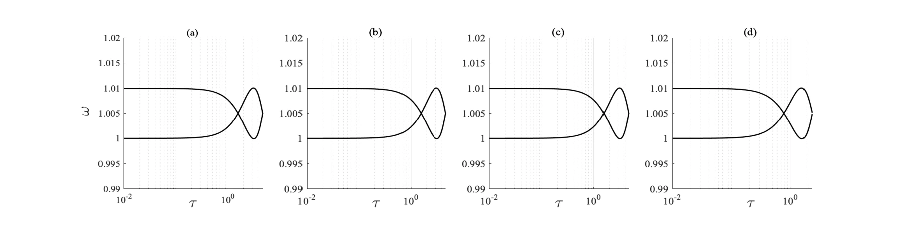
Compare the imaginary components.
The corresponding imaginary components describe the oscillatory part of the modes. Viewing them alongside the real components exposes differences between methods that a single stability metric could miss.
Panels (a)–(d). The same method order is retained for the imaginary components, allowing each solver’s frequency branches to be read alongside its real-part result.
Putting it together
Choose a solver by the dynamics it must resolve.
Using the same oscillator model makes the numerical methods directly comparable. Real and imaginary eigenvalue components provide complementary checks on the behavior predicted by each approximation.
Citation
Abdelrahman, A. S., Al-Qahtani, H. M., & Alharbi, F. H. A Comparison of Numerical Solvers for the Delay Eigenvalue Problem of Coupled Oscillators. Journal of Physics: Conference Series, 1730(1) (2021).
BibTeX
@article{abdelrahman2021delay,
  title = {A Comparison of Numerical Solvers for the Delay Eigenvalue Problem of Coupled Oscillators},
  author = {Abdelrahman, Abdelrahman S. and Al-Qahtani, Hussain and Alharbi, Fahhad H.},
  journal = {Journal of Physics: Conference Series},
  volume = {1730},
  number = {1},
  pages = {012114},
  year = {2021},
  doi = {10.1088/1742-6596/1730/1/012114}
}