The question
A hardware sampler rarely behaves like an ideal mathematical activation function. This work asks whether variational optimization can operate with the asymmetric responses and variability of real SPAD devices. The story moves from the physical platform to characterization, algorithm tests, and deeper simulated schedules.
Close the loop around a real array.
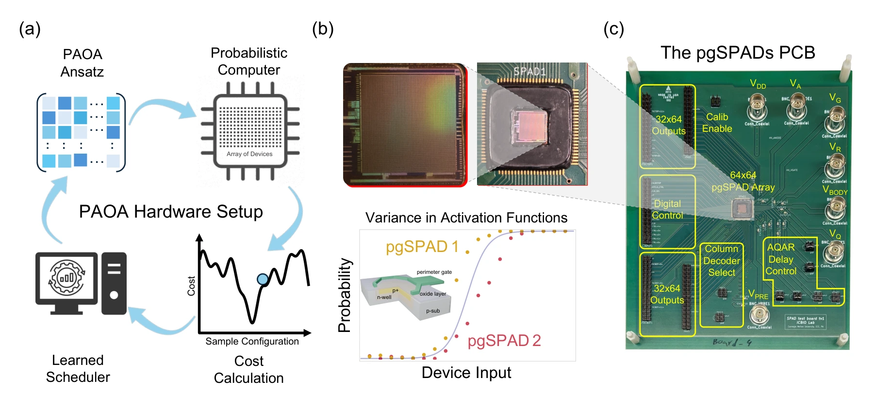
The hardware–software loop combines a classical optimizer, cost evaluations, and samples from a 64 × 64 perimeter-gated SPAD array. The chip and board photographs place the algorithm alongside the physical platform and its nonuniform device responses.
Panel (a). The optimizer receives a cost estimated from sampled configurations and updates the PAOA parameters. This is the algorithmic loop that the physical sampler supports.
Panels (b) and (c). The die view shows distinct device activation curves, while the board photograph places the array alongside its control and readout circuitry. Their separation makes device variability visible within the system architecture.
Turn avalanche events into probabilistic bits.
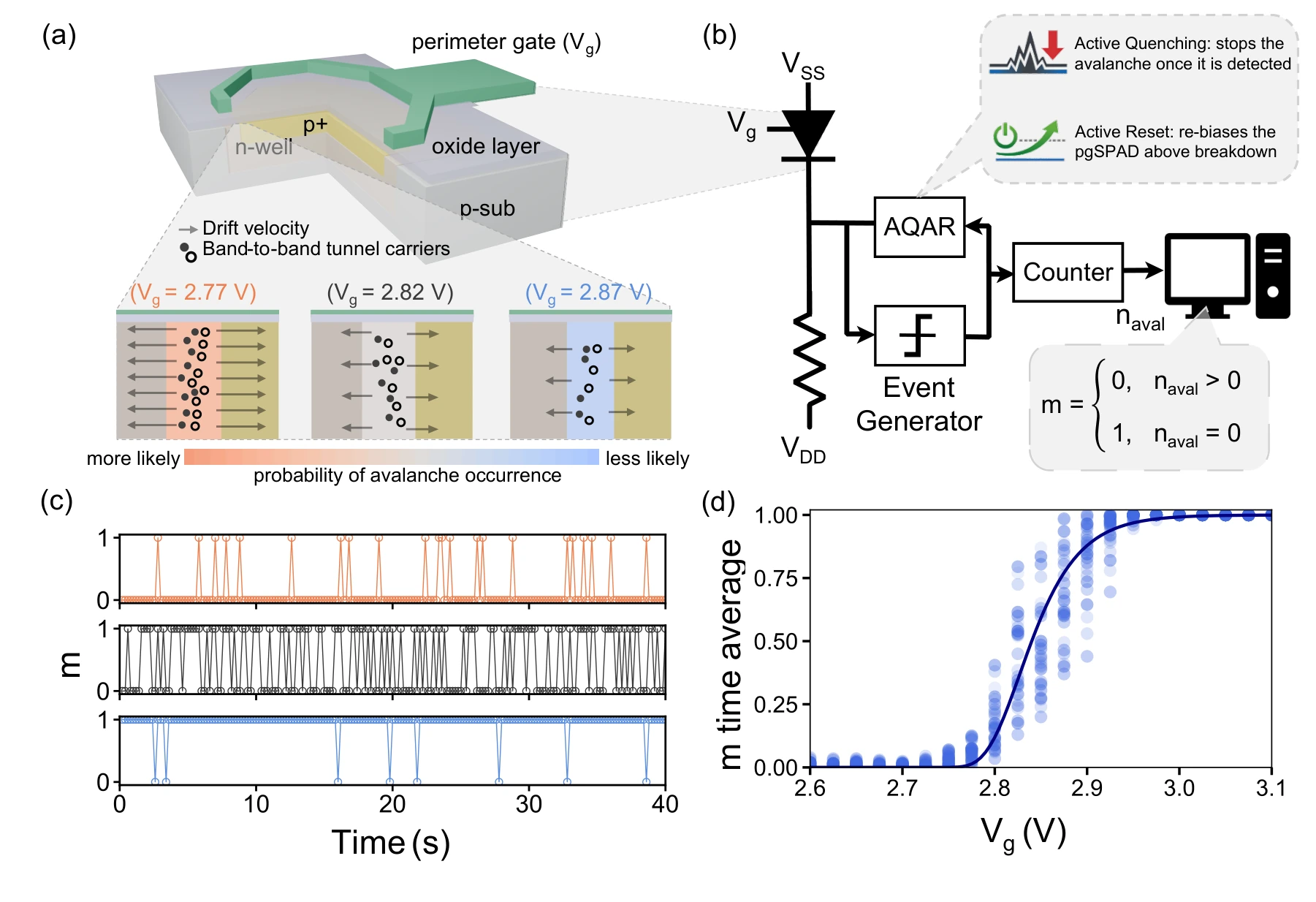
Gate voltage changes the dark-count behavior of each device. Quenching, reset, and a defined integration window turn those stochastic events into binary outputs; their averaged response reveals the activation function available to the algorithm.
Panels (a) and (b). The perimeter gate changes the electric field near the SPAD junction edge. The readout circuit then converts avalanche events into a bit: at least one event within the integration window gives one output state, while no event gives the other.
Panels (c) and (d). The time traces show how gate voltage changes switching statistics. The measured activation curves compare devices, rather than repeated measurements of one ideal element; the Gompertz fit describes their asymmetric average response.
Match the algorithm to the device response.
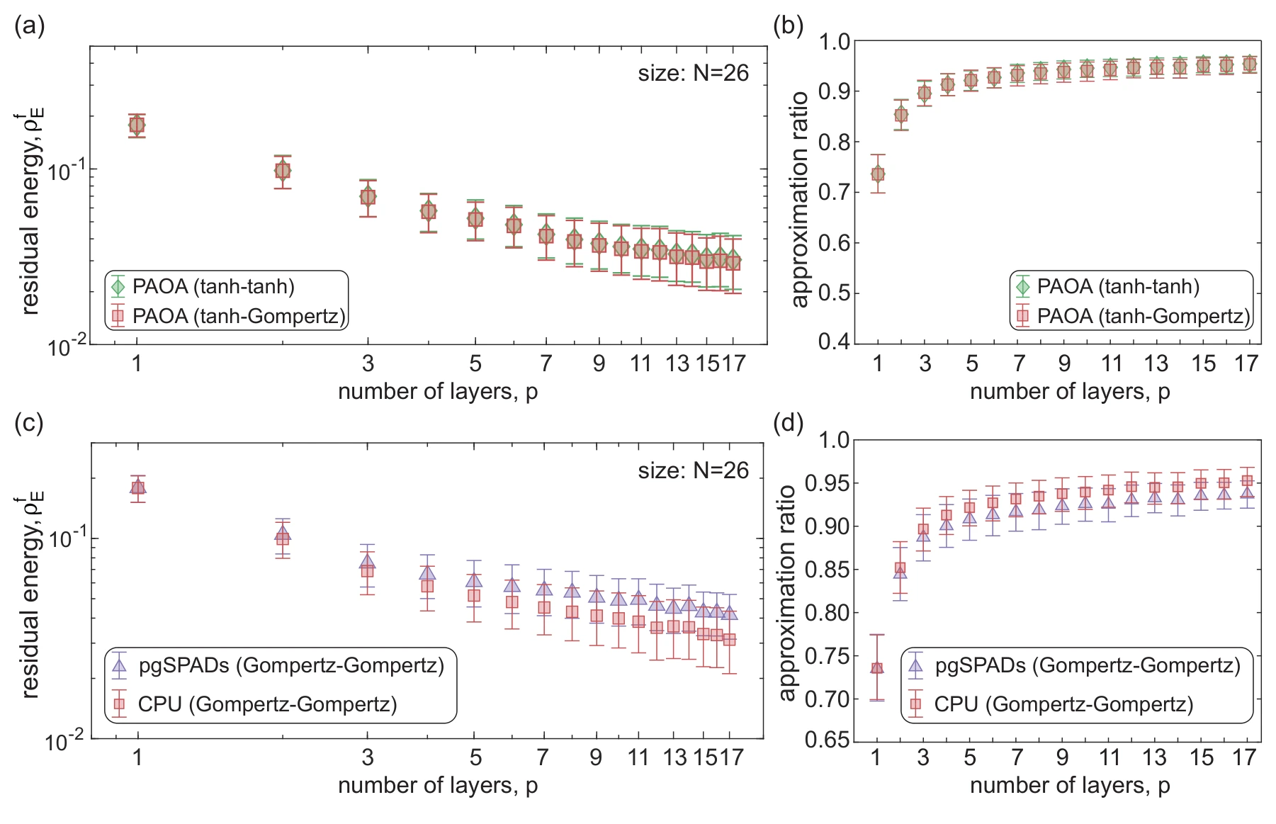
The benchmarks separate activation mismatch from matched hardware deployment. They compare idealized tanh and asymmetric Gompertz responses, then place measured SPAD inference alongside simulation using a hardware-matched training model.
Panels (a) and (b). Residual energy and approximation ratio compare matched tanh training/inference with tanh training followed by Gompertz inference. The schedules are learned on training instances and applied to a separate test set without retraining.
Panels (c) and (d). These panels instead use matched Gompertz schedules for both hardware and CPU inference. The hardware averages 50 runs, compared with one million in simulation. Bootstrap confidence intervals help distinguish agreement from sampling variability.
Ask what happens at greater depth.
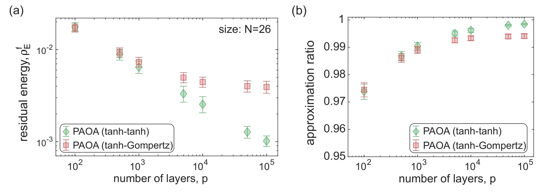
CPU simulations extrapolate schedules learned at shallow depth to much longer runs. Residual energy and approximation ratio track the resulting improvement. These large-depth curves are simulations, rather than additional measurements on the physical array.
Panels (a) and (b). The same extrapolated schedules are evaluated using residual energy and approximation ratio. They were learned at depth 17 and extended without retraining; these large-depth results are CPU simulations, with confidence intervals across the tested instances and runs.
Supplementary figures 7 figures
Compare the physical SPAD structures.
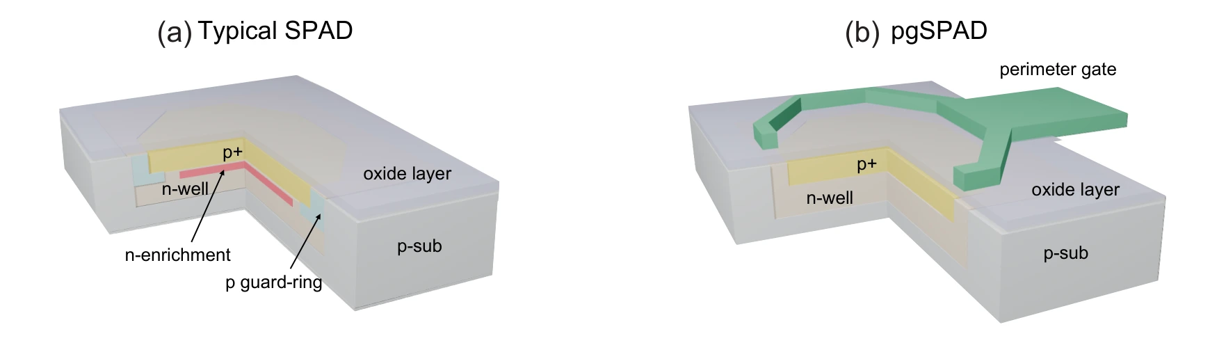
Cross-sections contrast a conventional SPAD with its perimeter-gated variant. The gate provides a way to influence the junction-edge electric field and the resulting stochastic behavior.
Panels (a) and (b). The cross-sections compare a conventional SPAD with the added perimeter gate. That gate provides a separate way to influence the junction-edge field.
Connect dark counts to operating conditions.
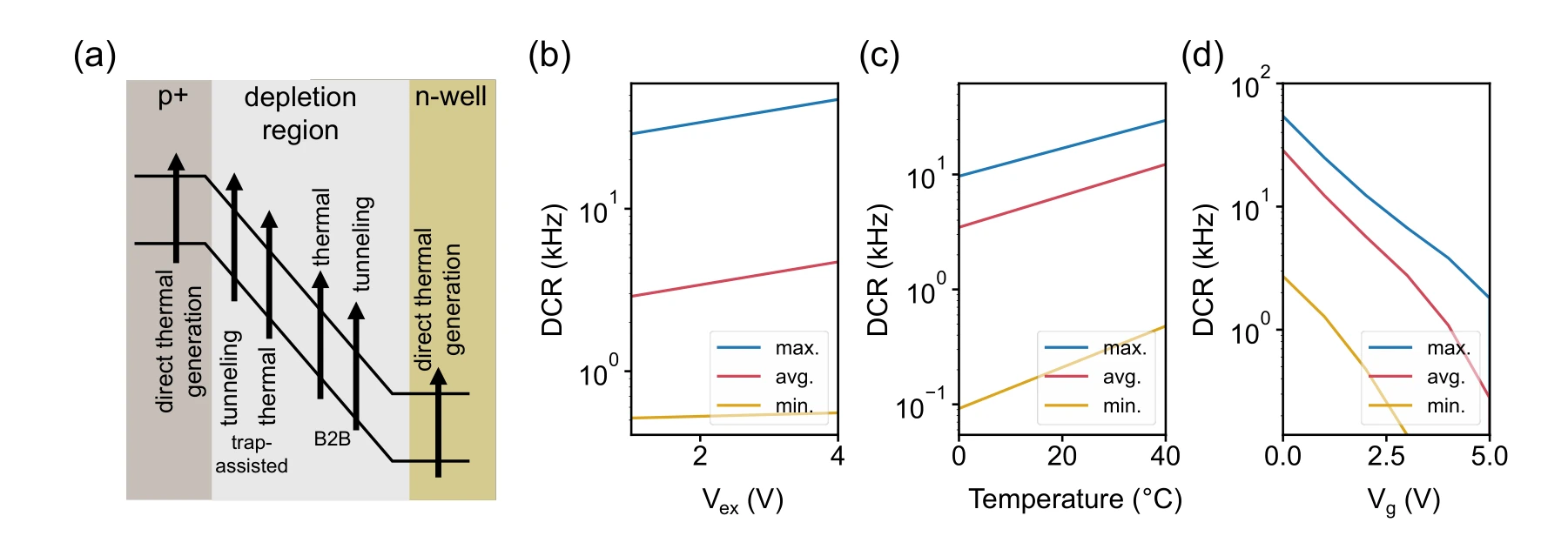
The panels relate carrier-generation mechanisms to bias voltage, temperature, and gate voltage. These measurements explain why a device’s probabilistic response changes with its environment.
Panel (a) and panels (b)–(d). Carrier-generation mechanisms are followed by measured dark-count rates versus excess bias, temperature, and gate voltage. Minimum, maximum, and mean curves expose variation across the array.
Inspect the chip and pixel architecture.
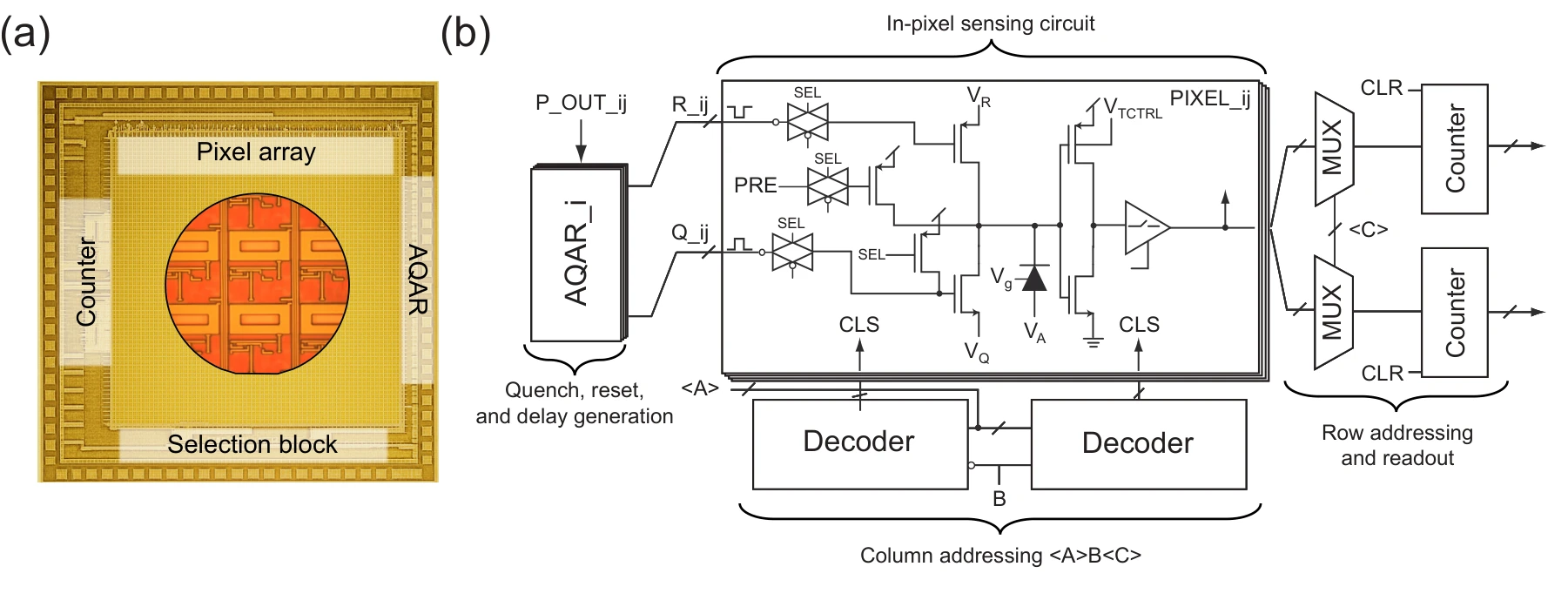
The photomicrograph and circuit schematic connect the 64 × 64 array to the addressing, quenching, reset, and readout functions required for characterization.
Panels (a) and (b). The micrograph identifies the array on the die. The circuit diagram shows the addressing, quench/reset, and counter blocks that make individual-pixel characterization possible.
Describe the asymmetric activation mathematically.
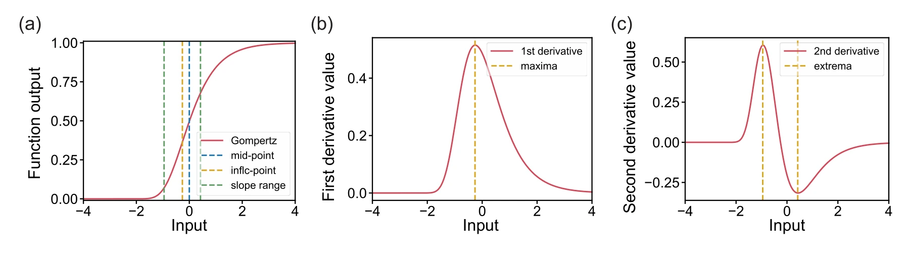
The Gompertz response and its derivatives identify the midpoint, inflection point, and transition range. They provide interpretable quantities for modeling the measured activation curves.
Panels (a)–(c). The activation curve and its first two derivatives distinguish the midpoint, inflection point, and transition range of the asymmetric Gompertz response.
Separate fabrication variation from operating shifts.
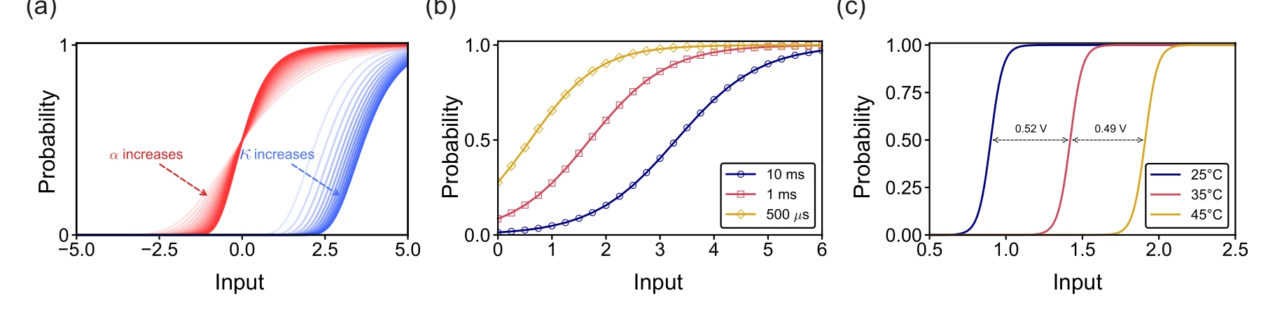
Simulations and measurements show how slope and midpoint change across device parameters, integration windows, and temperature. These effects motivate activation-aware learning.
Panels (a)–(c). Simulation separates slope changes from midpoint shifts. Measurements then show how integration time and temperature alter the effective activation curve, alongside manufacturing variability.
Document the characterization apparatus.
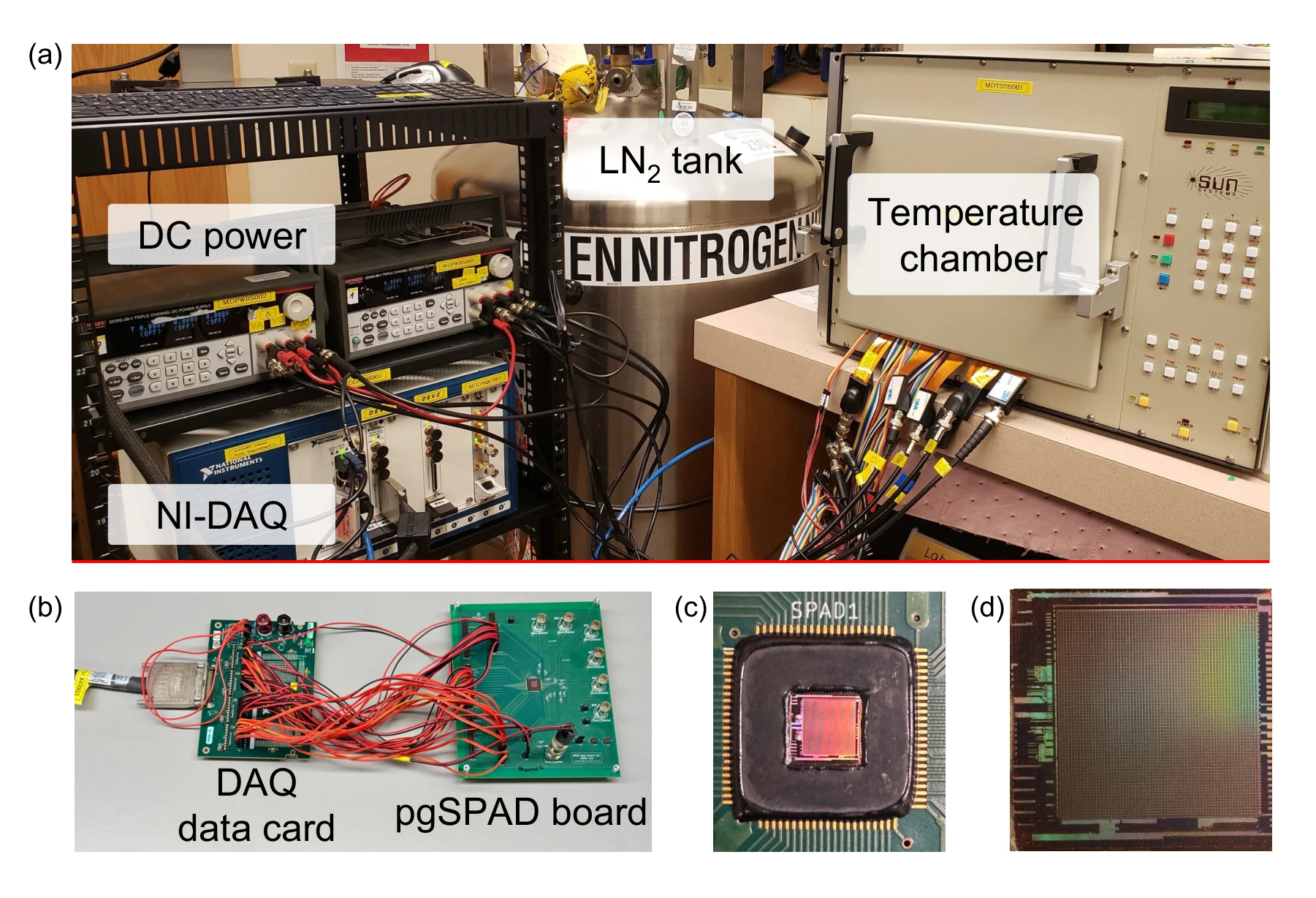
The temperature chamber, data-acquisition equipment, board, and die connect the reported device responses to the actual measurement setup.
Panels (a) and (b). The temperature chamber, liquid-nitrogen tank, and power supplies establish the operating conditions. The data-acquisition setup supplies timing signals and records the device output, connecting the characterization curves to a physical measurement procedure.
Panels (c) and (d). The board photograph shows the wire-bonded chip and protected connections. The micrograph locates the 64 × 64 array and its peripheral logic. These are different views of the same measurement platform, from laboratory equipment down to the die.
Return to a small, inspectable learning problem.
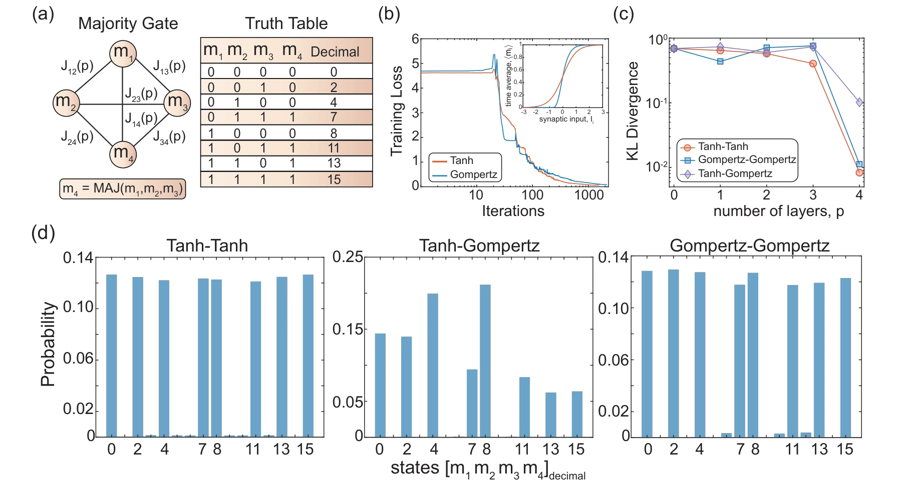
A majority-gate benchmark compares matched tanh and Gompertz learning with mismatched inference. The loss, divergence, and final state distributions make the effect of activation choice visible.
Panels (a) and (b). The majority-gate network and its valid truth-table states define an exactly inspectable target. The training curves then compare learning with symmetric tanh and asymmetric Gompertz activations.
Panels (c) and (d). KL divergence and the final state probabilities distinguish matched training/inference from activation mismatch. Comparing these two panels checks both a scalar error measure and which configurations receive probability at the final depth.
Putting it together
Learning with device characteristics.
The experiments connect device characterization to the optimization procedure. They support using a model of the hardware response during learning instead of assuming that every physical stochastic element implements an ideal tanh function.
Citation
Alswaidan, Z., Abdelrahman, A. S., Sajal, M. S., Chowdhury, S., Lin, K.-C., Guthrie, H., Seshan, S., Blanton, S., Morone, F., Dandin, M., Camsari, K. Y., & Srimani, T. Probabilistic approximate optimization using single-photon avalanche diode arrays. npj Unconventional Computing, in press (2026).
BibTeX
@article{alswaidan2026spad,
  title = {Probabilistic approximate optimization using single-photon avalanche diode arrays},
  author = {Alswaidan, Ziyad and Abdelrahman, Abdelrahman S. and Sajal, Md Sakibur and Chowdhury, Shuvro and Lin, Kai-Chun and Guthrie, Hunter and Seshan, Sanjay and Blanton, Shawn and Morone, Flaviano and Dandin, Marc and Camsari, Kerem Y. and Srimani, Tathagata},
  journal = {npj Unconventional Computing},
  year = {2026},
  note = {In press},
  eprint = {2602.13943},
  archivePrefix = {arXiv},
  url = {https://arxiv.org/abs/2602.13943}
}